This week we discussed Stochastic variational learning in recurrent spiking networks by Danilo Rezende and Wolfram Gerstner.
Introduction
This paper brings together variational inference (VI) and biophysical networks of spiking neurons. The authors show:
- variational learning can be implemented by networks of spiking neurons to learn generative models of data,
- learning takes the form of a biologically plausible learning rule, where local synaptic learning signals are augmented with a global “novelty” signal.
One potential application the authors mention is to use this method to identify functional networks from experimental data. Through the course of the paper, some bedrock calculations relevant to computational neuroscience and variational inference are performed. These include computing the log likelihood of a population of spiking neurons with Poisson noise (including deriving the continuum limit from discrete time) and derivation of the score function estimator. I’ve filled in some of the gaps in these derivations in this blog post (plus some helpful references I consulted) for anyone seeing this stuff for the first time.
Neuron model and data log likelihood
The neuron model used in this paper is the spike response model which the authors note (and we discussed at length) is basically a GLM. The membrane potential of each unit in the network is described by the following equation:
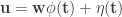
where 


Spikes are generated by defining an instantaneous firing rate ![\rho(t) = \rho_0 \text{exp}[\frac{\mathbf{u} - \theta}{\Delta u}]](https://s0.wp.com/latex.php?latex=%5Crho%28t%29+%3D+%5Crho_0+%5Ctext%7Bexp%7D%5B%5Cfrac%7B%5Cmathbf%7Bu%7D+-+%5Ctheta%7D%7B%5CDelta+u%7D%5D&bg=ffffff&fg=333333&s=0&c=20201002)


![[t,t+\Delta t]](https://s0.wp.com/latex.php?latex=%5Bt%2Ct%2B%5CDelta+t%5D&bg=ffffff&fg=333333&s=0&c=20201002)

![P_i(t_i^f \in [t,t+\Delta t] | \mathbf{X}(0...t)) \approx \rho_i(t) \Delta t](https://s0.wp.com/latex.php?latex=P_i%28t_i%5Ef+%5Cin+%5Bt%2Ct%2B%5CDelta+t%5D+%7C+%5Cmathbf%7BX%7D%280...t%29%29+%5Capprox+%5Crho_i%28t%29+%5CDelta+t&bg=ffffff&fg=333333&s=0&c=20201002)
![P_i(t_i^f \notin [t,t+\Delta t] | \mathbf{X}(0...t)) \approx 1 - \rho_i(t) \Delta t](https://s0.wp.com/latex.php?latex=P_i%28t_i%5Ef+%5Cnotin+%5Bt%2Ct%2B%5CDelta+t%5D+%7C+%5Cmathbf%7BX%7D%280...t%29%29+%5Capprox+1+-+%5Crho_i%28t%29+%5CDelta+t&bg=ffffff&fg=333333&s=0&c=20201002)
Aside: in future sections, the activity of some neurons will be observed (visible) and denoted by a super- or subscript 

We can define the joint probability of the entire set of spikes as:
![P(X(0...T)) \approx \Pi_{i \in \mathcal{V} \cup \mathcal{H}} \Pi_{k_i^s} [\rho_i(t^f_{k_i^s})\Delta t] \Pi_{k_i^{ns}} [1 - \rho_i(t^f_{k_i^{ns}})\Delta t]](https://s0.wp.com/latex.php?latex=P%28X%280...T%29%29+%5Capprox+%5CPi_%7Bi+%5Cin+%5Cmathcal%7BV%7D+%5Ccup+%5Cmathcal%7BH%7D%7D+%5CPi_%7Bk_i%5Es%7D+%5B%5Crho_i%28t%5Ef_%7Bk_i%5Es%7D%29%5CDelta+t%5D+%5CPi_%7Bk_i%5E%7Bns%7D%7D+%5B1+-+%5Crho_i%28t%5Ef_%7Bk_i%5E%7Bns%7D%7D%29%5CDelta+t%5D&bg=ffffff&fg=333333&s=0&c=20201002)
The authors re-express this in the continuum limit. A detailed explanation of how to do this can be found in Abbott and Dayan, Chapter 1, Appendix C. The key is to expand the log of the “no spike” term into a Taylor series, truncate at the first term and then exponentiate it:
![\text{exp} \hspace{1mm} \text{log} (\Pi_{k_i^{ns}} [1 - \rho_i(t^f_{k_i^{ns}})\Delta t]) = \text{exp} \sum_{k_i^{ns}} \text{log} [1 - \Delta t \rho_i(t_{k_i^{ns}}^f)] \approx \text{exp} \sum_{k_i^{ns}} - \Delta t \rho_i(t_{k_i^{ns}}^f)](https://s0.wp.com/latex.php?latex=%5Ctext%7Bexp%7D+%5Chspace%7B1mm%7D+%5Ctext%7Blog%7D+%28%5CPi_%7Bk_i%5E%7Bns%7D%7D+%5B1+-+%5Crho_i%28t%5Ef_%7Bk_i%5E%7Bns%7D%7D%29%5CDelta+t%5D%29+%3D+%5Ctext%7Bexp%7D+%5Csum_%7Bk_i%5E%7Bns%7D%7D+%5Ctext%7Blog%7D+%5B1+-+%5CDelta+t+%5Crho_i%28t_%7Bk_i%5E%7Bns%7D%7D%5Ef%29%5D+%5Capprox+%5Ctext%7Bexp%7D+%5Csum_%7Bk_i%5E%7Bns%7D%7D+-+%5CDelta+t+%5Crho_i%28t_%7Bk_i%5E%7Bns%7D%7D%5Ef%29&bg=ffffff&fg=333333&s=0&c=20201002)
As 
![P(\mathbf{X}(0...T)) = \Pi_{i \in \mathcal{V} \cup \mathcal{H}} [\Pi_{t_i^f}\rho_i(t_i^f) \Delta t] \text{exp}(- \int_0^T dt \rho_i(t))](https://s0.wp.com/latex.php?latex=P%28%5Cmathbf%7BX%7D%280...T%29%29+%3D+%5CPi_%7Bi+%5Cin+%5Cmathcal%7BV%7D+%5Ccup+%5Cmathcal%7BH%7D%7D+%5B%5CPi_%7Bt_i%5Ef%7D%5Crho_i%28t_i%5Ef%29+%5CDelta+t%5D+%5Ctext%7Bexp%7D%28-+%5Cint_0%5ET+dt+%5Crho_i%28t%29%29&bg=ffffff&fg=333333&s=0&c=20201002)
from which we can compute the log likelihood,
![\text{log} P(\mathbf{X}(0...T) = \sum_{i \in \mathcal{V} \cup \mathcal{H}} \int_0^T d\tau [\text{log} \rho_i(\tau) \mathbf{X}_i(\tau) - \rho_i(\tau)]](https://s0.wp.com/latex.php?latex=%5Ctext%7Blog%7D+P%28%5Cmathbf%7BX%7D%280...T%29+%3D+%5Csum_%7Bi+%5Cin+%5Cmathcal%7BV%7D+%5Ccup+%5Cmathcal%7BH%7D%7D+%5Cint_0%5ET+d%5Ctau+%5B%5Ctext%7Blog%7D+%5Crho_i%28%5Ctau%29+%5Cmathbf%7BX%7D_i%28%5Ctau%29+-+%5Crho_i%28%5Ctau%29%5D&bg=ffffff&fg=333333&s=0&c=20201002)
where we use 
They note that this equation is not a sum of independent terms, since 
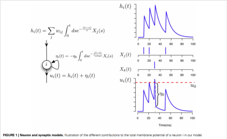
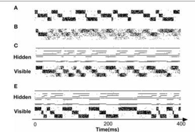
Figure 2 from the paper show the relevant network structures we will focus on. Panel C shows the intra- and inter- network connectivity between and among the hidden and visible units. Panel D illustrates the connectivity for the “inference” 

Variational Inference with stochastic gradients
From here, they follow a pretty straightforward application of VI. I will pepper my post with terms we’ve used/seen in the past to make these connections as clear as possible. They construct a recurrent network of spiking neurons where the spiking data of a subset of the neurons (the visible neurons or “the observed data”) can be explained by the activity of a disjoint subset of unobserved neurons (or a “latent variable” ala the VAE). Like standard VI, they want to approximate the posterior distribution of the spiking patterns of the hiding variables (like one would approximate the posterior of a latent variable in a VAE) by minimizing the KL-divergence between the true posterior and an approximate posterior 


The second term is the data log likelihood. The first term, 


where 
![\nabla_{w_{ij}^\mathcal{M}} \hat{\mathcal{L}}^\mathcal{M} = \nabla_{w_{ij}^\mathcal{M}} \text{log} p(\mathcal{X_H, X_V}) = \sum_{k \in \mathcal{V} \cup \mathcal{H}} \int_0^T d\tau \frac{\partial \text{log} \rho_k(\tau)}{\partial w_{ij}^\mathcal{M}} [\mathbf{X}_k(\tau) - \rho_k(\tau)]](https://s0.wp.com/latex.php?latex=%5Cnabla_%7Bw_%7Bij%7D%5E%5Cmathcal%7BM%7D%7D+%5Chat%7B%5Cmathcal%7BL%7D%7D%5E%5Cmathcal%7BM%7D+%3D+%5Cnabla_%7Bw_%7Bij%7D%5E%5Cmathcal%7BM%7D%7D+%5Ctext%7Blog%7D+p%28%5Cmathcal%7BX_H%2C+X_V%7D%29+%3D+%5Csum_%7Bk+%5Cin+%5Cmathcal%7BV%7D+%5Ccup+%5Cmathcal%7BH%7D%7D+%5Cint_0%5ET+d%5Ctau+%5Cfrac%7B%5Cpartial+%5Ctext%7Blog%7D+%5Crho_k%28%5Ctau%29%7D%7B%5Cpartial+w_%7Bij%7D%5E%5Cmathcal%7BM%7D%7D+%5B%5Cmathbf%7BX%7D_k%28%5Ctau%29+-+%5Crho_k%28%5Ctau%29%5D&bg=ffffff&fg=333333&s=0&c=20201002)
Here they used the handy identity: ![\frac{\partial f(x)}{\partial x} = \frac{\partial[\text{log} f(x)]}{\partial x} f(x)](https://s0.wp.com/latex.php?latex=%5Cfrac%7B%5Cpartial+f%28x%29%7D%7B%5Cpartial+x%7D+%3D+%5Cfrac%7B%5Cpartial%5B%5Ctext%7Blog%7D+f%28x%29%5D%7D%7B%5Cpartial+x%7D+f%28x%29&bg=ffffff&fg=333333&s=0&c=20201002)
The derivative of the firing rate function can be computed with the chain rule, ![\frac{\partial [\text{log} \rho_k(\tau)]}{\partial w_{ij}^\mathcal{M}} = \delta_{ki} \frac{g^\prime(u_k(\tau))}{g(u_k(\tau))} \phi_j(\tau)](https://s0.wp.com/latex.php?latex=%5Cfrac%7B%5Cpartial+%5B%5Ctext%7Blog%7D+%5Crho_k%28%5Ctau%29%5D%7D%7B%5Cpartial+w_%7Bij%7D%5E%5Cmathcal%7BM%7D%7D+%3D+%5Cdelta_%7Bki%7D+%5Cfrac%7Bg%5E%5Cprime%28u_k%28%5Ctau%29%29%7D%7Bg%28u_k%28%5Ctau%29%29%7D+%5Cphi_j%28%5Ctau%29&bg=ffffff&fg=333333&s=0&c=20201002)
This equation for updating the weights using gradient ascent is purely local, taking the form of a product between a presynaptic component, 
![\frac{g^\prime(u_k(\tau))}{g(u_k(\tau))} [\mathbf{X}_k(\tau) - \rho_k(\tau)]](https://s0.wp.com/latex.php?latex=%5Cfrac%7Bg%5E%5Cprime%28u_k%28%5Ctau%29%29%7D%7Bg%28u_k%28%5Ctau%29%29%7D+%5B%5Cmathbf%7BX%7D_k%28%5Ctau%29+-+%5Crho_k%28%5Ctau%29%5D&bg=ffffff&fg=333333&s=0&c=20201002)
They also compute the gradient of 

A cute proof of this can be found here. This comes in handy when computing the gradient of

Here again we compute Monte Carlo estimators of 


Reducing gradient estimation variance
The authors note that the stochastic gradient they introduced has been used extensively in reinforcement learning and that its variance is prohibitively high. To deal with this (presumably following the approach others have developed in RL, vice versa) they adopt a simple, baseline removal approach. They subtract the mean 


Numerical results
Details of their numerical simulations:
- Training data is binary arrays of spike data.
- Training data comes in batches of 200 ms with 500 batches sequentially shown to the network (100 s of data).
- During learning, visible neurons are forced to spike like the training data.
- Log likelihood of test data was estimated with importance sampling. Given a generative model with density
, importance sampling allows us to estimate the density of
:

![= \langle \text{exp}[\text{log}p(x_v,x_h) - \text{log} q(x_h|x_v)] \rangle_q = \langle \text{exp}[-\hat{\mathcal{F}}(x_v,x_h)]\rangle_{q(x_v|x_h)}](https://s0.wp.com/latex.php?latex=%3D+%5Clangle+%5Ctext%7Bexp%7D%5B%5Ctext%7Blog%7Dp%28x_v%2Cx_h%29+-+%5Ctext%7Blog%7D+q%28x_h%7Cx_v%29%5D+%5Crangle_q+%3D+%5Clangle+%5Ctext%7Bexp%7D%5B-%5Chat%7B%5Cmathcal%7BF%7D%7D%28x_v%2Cx_h%29%5D%5Crangle_%7Bq%28x_v%7Cx_h%29%7D&bg=ffffff&fg=333333&s=0&c=20201002)
Using this equation, they estimate the log likelihood of the observed spike trains by sampling several times from the
Here is an example of training with this method with 50 hidden units using the “stairs” dataset. C shows that the network during the “sleep phase” (running in generative mode) forms a latent representation of the stairs in the hidden layers. Running the network in “inference mode” (wake, in the wake-sleep parlance), when the
Role of the novelty signal
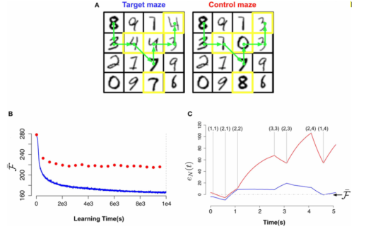
To examine the role of the novelty signal, they train a network to perform a maze task. Each maze contains 16 rooms where each room is a 28×28 pixel greyscale image of a MNIST digit. Each room is only accessible from a neighboring room. Pixel values were converted into firings rates from 0.01 to 9 Hz. In the test maze (or control maze), some of the rooms of the training maze were changed. The network had 28×28 visible units and 30 hidden units. These were recurrent binary units. Data were generated from random trajectories of 100 time steps in the target maze. Each learning epoch was 500 presentations of the data batches.
Below, (bottom left) they plotted the slow moving average of the free energy
Bottom right shows the free energy error signal for the sample trajectory in A. It fluctuates near zero for the learned maze but deviates largely for the test maze. We can see at (3,3) the free energy signal really jump up, meaning that the model identifies this as different from the target.
To conclude, the authors speculate that a neural correlate of this free energy error signal should look like an activity burst when an animal traverses unexpected situations. Also, they expect to see a substantial increase in the variance of the changes in synaptic weights when moving from a learned to a unfamiliar maze due to the change in the baseline of surprise levels.