
A few weeks ago in lab meeting we discussed ‘Organizing recurrent network dynamics by task-computation to enable continual learning’ by Duncker & Driscoll et. al 2020. This paper seeks to understand how a neural population maintains the flexibility to learn new tasks while robustly executing previously learned tasks. While biological networks learn new tasks all the time in a sequential (a.k.a. continual) fashion, continual learning in artificial neural networks has proven to be hard. These networks are known to catastrophically forget previous tasks when trained on a new task. In this work, the authors come up with a learning rule that enables a recurrent neural network to learn multiple tasks sequentially without catastrophic forgetting.
Let’s first formally define continual learning: We want to train a model on K tasks sequentially, where each task has its own set of input/output pairs represented by 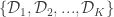
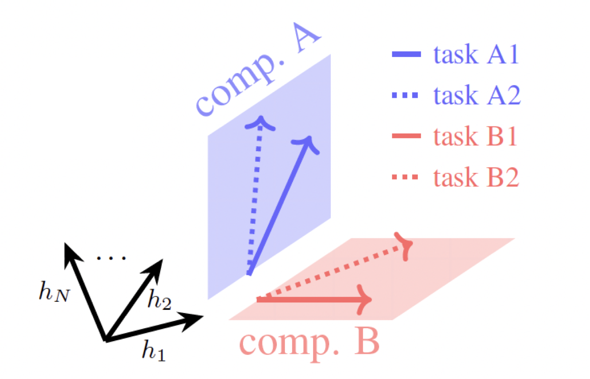
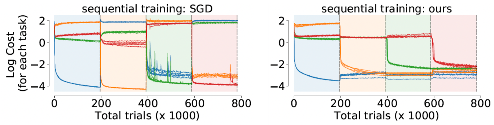
Continual learning for recurrent neural networks: This paper aims to perform continual learning using recurrent neural networks (RNNs), which are often studied as proxies for neural populations in neuroscience. The intuition behind their approach is to allow tasks that require similar computations/dynamics to use shared subspaces, while tasks that require different computations and would otherwise interfere with previously learned are encouraged to use an orthogonal subspace (see figure above).
They consider RNNs of the following form:

where 


![W = [W^{rec}, W^{in}]](https://s0.wp.com/latex.php?latex=W+%3D+%5BW%5E%7Brec%7D%2C+W%5E%7Bin%7D%5D&bg=ffffff&fg=333333&s=0&c=20201002)


and 
Project, and then project again: The authors modify this update rule such that:
Here, 
![z_t^{k,r}=[h_t^{k,r}, x_t^{k,r}]](https://s0.wp.com/latex.php?latex=z_t%5E%7Bk%2Cr%7D%3D%5Bh_t%5E%7Bk%2Cr%7D%2C+x_t%5E%7Bk%2Cr%7D%5D&bg=ffffff&fg=333333&s=0&c=20201002)


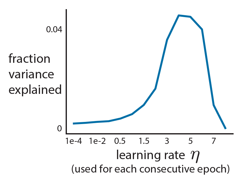
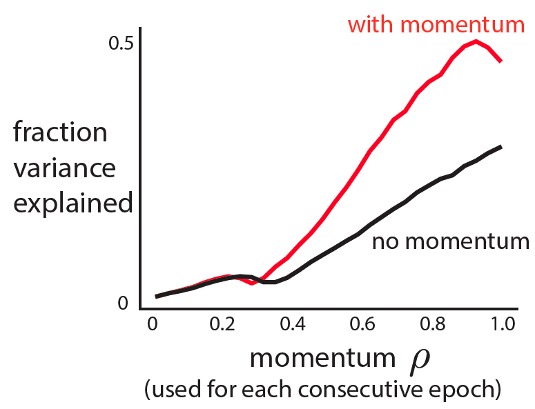
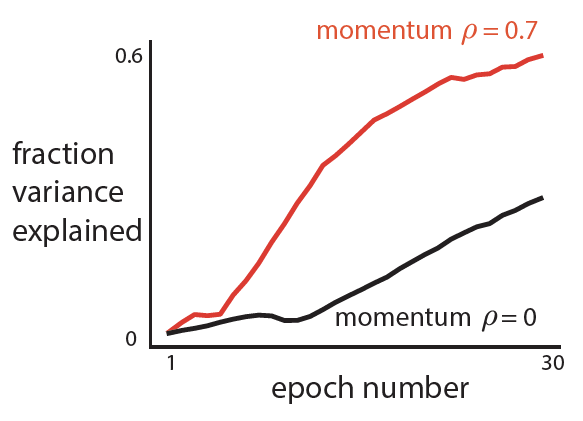
It works! They test their method on a set of four neuroscience tasks (from Yang et al. 2019). The key results without going into task details are as follows:
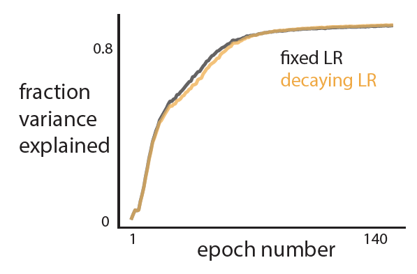
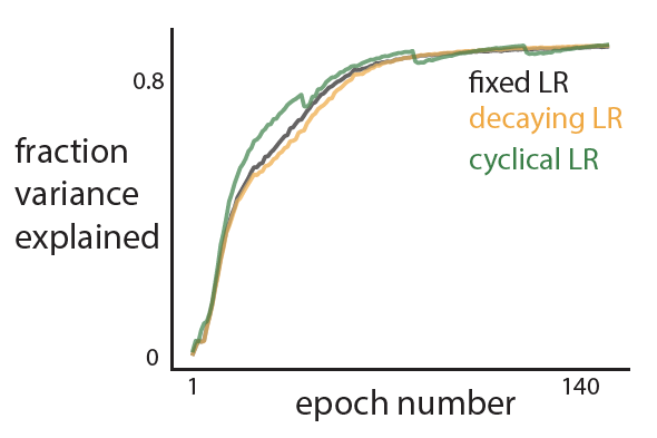
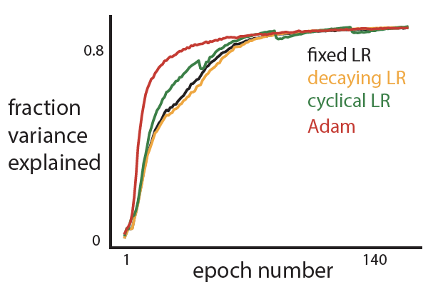
- Their approach is able to train a network sequentially on all the 4 tasks with better test performance across tasks as compared to existing methods and standard SGD (see figure; each color represents a new task).
- They find that the underlying dynamics of hidden states of the network (near fixed points) for a task remains fixed even after the network is trained on newer tasks, showing that their training procedure is indeed robust!
- They find empirical evidence that dynamics corresponding to some tasks evolve in shared subspaces (of the high-dimensional hidden states), while others use orthogonal subspaces.
- They find organizational differences between learned dynamics through sequential training and simultaneous training: simultaneous training results in slightly better results and more efficient usage of shared structure across tasks.
Questions for future research: An important question that this approach raises is whether there is an upper limit to the number of dissimilar tasks that such a learning rule can enable the network to learn. How long can we keep projecting away from the space of outputs and inputs? Furthermore, how much does the order of tasks matter as the dynamics corresponding to newer tasks can only occupy the remaining orthogonal subspace? And finally the million dollar question: how do real neurons in the brain learn new tasks sequentially?
 , they considered spikes from unit
  until either a response
  was made at time
  , or to the end of time window
  , whichever had come first, i.e., up to
  . The reason for restricting the trial duration accordingly had been to model the neural processes that led to behavioral responses, rather than what happened post-response. To handle the variability of
  across different trials, they proposed to re-scale the original spike times
  using a trial-specific monotonic function
 ![z_n: [0,W_n] \rightarrow [0,W]](https://s0.wp.com/latex.php?latex=z_n%3A+%5B0%2CW_n%5D+%5Crightarrow+%5B0%2CW%5D&bg=ffffff&fg=333333&s=0&c=20201002) ,
,  . Following this transformation, the latent neural
  given by
  , where
  is the stimulus embedding, can be related to the corresponding canonical (trial independent) intensity function
  by
by  . This facilitates the estimation of a single function
  .
. that was presented at trial
  in the form of the cumulative intensity function
  . The neural intensity function
  is then obtained by differentiating
  for making each action
  at each time
  to train all the weights from stimulus to neural cumulative intensity functions (blue and red rectangles in the following figure):
  , where
 ![\mathcal{L}^N_{u.n} = \sum_{i=1}^{|S_{u.n}|} \left[ \log \frac{\partial \Lambda^{N}_u(t= z_n(s_{u.n}^i);\mathbf{h}_n)}{\partial t}\right] - \frac{W_n}{W} \Lambda^{N}_u(W;\mathbf{h}_n)](https://s0.wp.com/latex.php?latex=%5Cmathcal%7BL%7D%5EN_%7Bu.n%7D+%3D+%5Csum_%7Bi%3D1%7D%5E%7B%7CS_%7Bu.n%7D%7C%7D+%5Cleft%5B+%5Clog+%5Cfrac%7B%5Cpartial+%5CLambda%5E%7BN%7D_u%28t%3D+z_n%28s_%7Bu.n%7D%5Ei%29%3B%5Cmathbf%7Bh%7D_n%29%7D%7B%5Cpartial+t%7D%5Cright%5D+-+%5Cfrac%7BW_n%7D%7BW%7D+%5CLambda%5E%7BN%7D_u%28W%3B%5Cmathbf%7Bh%7D_n%29&bg=ffffff&fg=333333&s=0&c=20201002) , and
, and  is the spike time relative to the stimulus onset of the
  spiking event of unit
 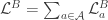 , where
  , and
, and  is the set of trials on which action
  was taken before


 , even when the number of samples (n) is less than the number of features or dimensions (d).
 ![r^2 = 1- \frac{E[(y-\beta^Tx)^2]}{E[y^2]}](https://s0.wp.com/latex.php?latex=r%5E2+%3D+1-+%5Cfrac%7BE%5B%28y-%5Cbeta%5ETx%29%5E2%5D%7D%7BE%5By%5E2%5D%7D&bg=ffffff&fg=333333&s=0&c=20201002)
 is the (scalar) output,
  is the vector (
 ) of regressors, and
  is the optimal least squares weight vector.
 is the least squares solution estimated on
  , thus your model wouldn’t actually achieve this performance on held-out data.
  , this is because your regressand matrix (x) is over-complete and there is no unique least-squares solution and if you regularize you can fit the data arbitrarily well (leaving no residuals on which to estimate performance).
![E[x_1y_1] =\beta](https://s0.wp.com/latex.php?latex=E%5Bx_1y_1%5D++%3D%5Cbeta&bg=ffffff&fg=333333&s=0&c=20201002)
![\beta = E[xx^T]^{-1} E[yx] = \Sigma_x^{-1} \Sigma_{x,y}](https://s0.wp.com/latex.php?latex=%5Cbeta+%3D+E%5Bxx%5ET%5D%5E%7B-1%7D+E%5Byx%5D+%3D+%5CSigma_x%5E%7B-1%7D+%5CSigma_%7Bx%2Cy%7D&bg=ffffff&fg=333333&s=0&c=20201002) . And with two independent observations of x and y, I can have:
. And with two independent observations of x and y, I can have:![E[(x_1y_1)^Tx_2y_2] = E[x_1y_1]^T E[x_2y_2] = \beta^T \beta](https://s0.wp.com/latex.php?latex=E%5B%28x_1y_1%29%5ETx_2y_2%5D+%3D+E%5Bx_1y_1%5D%5ET+E%5Bx_2y_2%5D+%3D+%5Cbeta%5ET+%5Cbeta++&bg=ffffff&fg=333333&s=0&c=20201002) .
. with an unbiased numerator and denominator.
![\mathcal{F(\mathbf{\theta})} := \int p(x; \theta)f(x; \phi)dx = \mathop{\mathbb{E}}_{p(x; \theta)}\Big[f(x; \phi)\Big] \qquad (1) \bigskip](https://s0.wp.com/latex.php?latex=%5Cmathcal%7BF%28%5Cmathbf%7B%5Ctheta%7D%29%7D+%3A%3D+%5Cint+p%28x%3B+%5Ctheta%29f%28x%3B+%5Cphi%29dx+%3D+%5Cmathop%7B%5Cmathbb%7BE%7D%7D_%7Bp%28x%3B+%5Ctheta%29%7D%5CBig%5Bf%28x%3B+%5Cphi%29%5CBig%5D+%5Cqquad+%281%29+%5Cbigskip&bg=ffffff&fg=333333&s=0&c=20201002)
 for which we do have a closed form evaluation), and or issues regarding the large space of values that variables of interest can take, thus making approximation by quadrature ineffective. These reasons tell us we will need some other type of approximation. That approximation will be a Monte Carlo estimator of the expectation. Generally we can define this estimator, given samples
  for
for  as (note that we are using approximately below to guide intuition, this is not the usual use of it):
![\mathop{\mathbb{E}}_{p(x; \theta)}\Big[f(x; \phi)\Big] \approx \mathcal{\bar F}_N = \bigskip \frac{1}{N} \sum_{n=1}^N f\Big(\hat x^{(n)} \Big) \qquad (2)](https://s0.wp.com/latex.php?latex=%5Cmathop%7B%5Cmathbb%7BE%7D%7D_%7Bp%28x%3B+%5Ctheta%29%7D%5CBig%5Bf%28x%3B+%5Cphi%29%5CBig%5D+%5Capprox+%5Cmathcal%7B%5Cbar+F%7D_N+%3D+%5Cbigskip+%5Cfrac%7B1%7D%7BN%7D+%5Csum_%7Bn%3D1%7D%5EN+f%5CBig%28%5Chat+x%5E%7B%28n%29%7D+%5CBig%29+%5Cqquad+%282%29&bg=ffffff&fg=333333&s=0&c=20201002)
 . One way to learn such parameters is through gradient descent. So we will need the gradient of the objective (which we have defined above as the expectation), which is (as usual):
![\nabla_{\theta}\mathbb{E}_{p(x; \theta)}[f(x; \phi)] \qquad (3)](https://s0.wp.com/latex.php?latex=%5Cnabla_%7B%5Ctheta%7D%5Cmathbb%7BE%7D_%7Bp%28x%3B+%5Ctheta%29%7D%5Bf%28x%3B+%5Cphi%29%5D+%5Cqquad+%283%29&bg=ffffff&fg=333333&s=0&c=20201002)
 . Thus it is (by the chain rule of differentiation):

![\nabla_{\theta} \mathbb{E}_{p(x; \theta)}[f(x; \phi)] = \nabla_{\theta} \int p(x; \theta)f(x; \phi) dx = \int f(x; \phi) \nabla_{\theta}p(x; \theta) dx \qquad (4)](https://s0.wp.com/latex.php?latex=%5Cnabla_%7B%5Ctheta%7D+%5Cmathbb%7BE%7D_%7Bp%28x%3B+%5Ctheta%29%7D%5Bf%28x%3B+%5Cphi%29%5D+%3D+%5Cnabla_%7B%5Ctheta%7D+%5Cint+p%28x%3B+%5Ctheta%29f%28x%3B+%5Cphi%29+dx+%3D+%5Cint+f%28x%3B+%5Cphi%29+%5Cnabla_%7B%5Ctheta%7Dp%28x%3B+%5Ctheta%29+dx+%5Cqquad+%284%29&bg=ffffff&fg=333333&s=0&c=20201002)
 , and the gradient does not in general satisfy the conditions to be considered a proper probability (e.g. the gradient can be negative!). However, due to the expression given by the definition of the score function, we can replace
  . Plugging this back in the the right most side of (4) we have:
![\int f(x; \phi)p(x; \theta)\nabla_{\theta} \log p(x; \theta) = \int p(x; \theta) [f(x; \phi) \nabla_{\theta} \log p(x; \theta)] = \mathbb{E}_{p(x; \theta)} [f(x; \phi)\nabla_{\theta} \log p(x; \theta)]](https://s0.wp.com/latex.php?latex=%5Cint+f%28x%3B+%5Cphi%29p%28x%3B+%5Ctheta%29%5Cnabla_%7B%5Ctheta%7D+%5Clog+p%28x%3B+%5Ctheta%29+%3D+%5Cint+p%28x%3B+%5Ctheta%29+%5Bf%28x%3B+%5Cphi%29+%5Cnabla_%7B%5Ctheta%7D+%5Clog+p%28x%3B+%5Ctheta%29%5D+%3D+%5Cmathbb%7BE%7D_%7Bp%28x%3B+%5Ctheta%29%7D+%5Bf%28x%3B+%5Cphi%29%5Cnabla_%7B%5Ctheta%7D+%5Clog+p%28x%3B+%5Ctheta%29%5D+&bg=ffffff&fg=333333&s=0&c=20201002)

 . The general reasoning behind why we’d want to do it, why it helps us achieve our goal is exactly the same as stated above. That is, when we take the gradient of the regular definition of the expectation, we no longer have an expectation. However for the reason of why’d you want to use the pathwise estimator over the score function we refer you to the original article. The name “pathwise” is motivated by two equivalent ways to sample a random variant from
  , and have used in the score function. The second and equivalent way to do this is by sampling a random variant from a simpler, continuous distribution:
  , and then transforming that variant via some function
  , that “encodes” the distributional parameters
  . The “path” version of sampling a random variant
  . Then we define the function :
 . So we have that
  , where
  , and the random variant is now
  . The form of this estimator is then:

 , when this is arbitrarily complex and may, for example, represent a distribution over all natural images. Alternatively, in the context of neuroscience,
  to a simpler probability distribution, such as a multivariate Gaussian distribution, over latent variable space
  . Assuming a bijective mapping
  , the Change of Variables formula is
 is the absolute value of the determinant of the Jacobian. This term is necessary so as to ensure probability mass is preserved during the transformation. In order to sample from
  can be converted into a sample from

 so as to ensure that
  operation, where
  is the dimension of

 , which are sampled from a multivariate normal distribution, to the target distribution. Here ‘
 ‘ denotes elementwise multiplication and
  and
and 

 -greedy exploration as has previously been suggested, lapses (errors on “easy” trials with strong sensory evidence) correspond to uncertainty-guided exploration. In particular, the authors compare empirically-obtained psychometric curves characterizing the performance of rats on a 2AFC task, with predicted psychometric curves from various normative models of lapses. They found that their softmax exploration model explains the empirical data best.
 is a sigmoidal curve (we will assume the cumulative normal distribution in what follows);
  determines the decision boundary and
  is the inverse slope parameter.
  is the lower asymptote of the curve, while
  is the upper asymptote. Together,
  , comprise the asymmetric lapse rates for the “easiest” stimuli (highest intensity stimuli).
  parameters of the psychometric curve.
  , the rat pays attention to the task-relevant stimulus, while, with probability
  , it ignores the stimulus and instead chooses according to its bias
  . That is:
 and
and  .
. ; the softmax-exploration model assumes that the animal chooses to go right in a 2AFC task according to
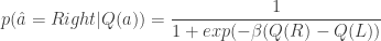
 is the difference in the expected value of choosing Right compared to choosing Left (see below). In the limit of
  , the animal will once again choose its action according to
  , where
  is the posterior distribution over the category of the stimulus (whether the frequency of the generated auditory and/or visual stimuli are above or below the predetermined threshold) given the animal’s noisy observations of the auditory and visual stimuli,
  and
and  .
.  is the reward the animal will obtain if it chooses to go Right and is correct. Similarly,
  .
.  and
and 
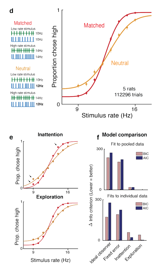

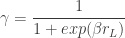
 greedy exploration are overly-simplistic. The asymmetric effect on left and right lapse rates of modified reward is particularly interesting, as many traditional models of lapses fail to capture this effect. Another contribution that this paper makes is in implicating the posterior striatum and secondary motor cortex as areas which may be involved in determining lapse rates; and better characterizing the role of these areas in lapse behavior than has been done in previous experiments.
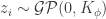
 , as
, as 
 is the post-activation of the jth neuron in the hidden layer;
  is some nonlinearity, and
  is the kth input to the network.
  ,
, 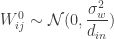 ; and that the biases are similarly sampled:
  and
and  ; then it is possible to show that, in the limit of
  ,
,  , for a kernel
  which depends on the nonlinearity. In particular, this follows from application of the Central Limit Theorem: for a fixed input to the network
  ,
,  as
as ![V_{\phi}(x^{1}(\vec{x})) \equiv \mathbb{E}[(x^{1}_{i}(\vec{x}))^{2}]](https://s0.wp.com/latex.php?latex=V_%7B%5Cphi%7D%28x%5E%7B1%7D%28%5Cvec%7Bx%7D%29%29+%5Cequiv+%5Cmathbb%7BE%7D%5B%28x%5E%7B1%7D_%7Bi%7D%28%5Cvec%7Bx%7D%29%29%5E%7B2%7D%5D&bg=ffffff&fg=333333&s=0&c=20201002) (which is the same for all
(which is the same for all  ).
).  . Application of the Multidimensional Central Limit Theorem tells us that, in the limit of
  ,
,  and
and 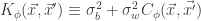 and
and ![C_{\phi}(\vec{x}, \vec{x'}) \equiv \mathbb{E}[x_{i}^{1}(\vec{x})x_{i}^{1}(\vec{x}')]](https://s0.wp.com/latex.php?latex=C_%7B%5Cphi%7D%28%5Cvec%7Bx%7D%2C+%5Cvec%7Bx%27%7D%29+%5Cequiv+%5Cmathbb%7BE%7D%5Bx_%7Bi%7D%5E%7B1%7D%28%5Cvec%7Bx%7D%29x_%7Bi%7D%5E%7B1%7D%28%5Cvec%7Bx%7D%27%29%5D&bg=ffffff&fg=333333&s=0&c=20201002) .
. 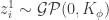 , as this is the very definition of a Gaussian process.
 th layer of a network with a Gaussian prior over all of the weights and biases is a sample from a Gaussian process in the limit of
  . They use an inductive argument of the form: suppose that
  (the jth output of the
  th layer of the network is sampled from a Gaussian process). Then:
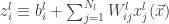
 will have a joint multivariate Gaussian distribution, i.e.,
  where
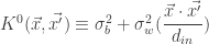
where ![K_{\phi}^{l}(\vec{x}, \vec{x'}) \equiv \mathbb{E}[z_{i}^{l}(\vec{x})z_{i}^{l}(\vec{x'})] = \sigma_{b}^{2} + \sigma_{w}^{2} \mathbb{E}_{z_{i}^{l-1}\sim \mathcal{GP}(0, K_{\phi}^{l-1})}[\phi(z_{i}^{l-1}(\vec{x})) \phi(z_{i}^{l-1}(\vec{x'}))]](https://s0.wp.com/latex.php?latex=K_%7B%5Cphi%7D%5E%7Bl%7D%28%5Cvec%7Bx%7D%2C+%5Cvec%7Bx%27%7D%29+%5Cequiv+%5Cmathbb%7BE%7D%5Bz_%7Bi%7D%5E%7Bl%7D%28%5Cvec%7Bx%7D%29z_%7Bi%7D%5E%7Bl%7D%28%5Cvec%7Bx%27%7D%29%5D+%3D+%5Csigma_%7Bb%7D%5E%7B2%7D+%2B+%5Csigma_%7Bw%7D%5E%7B2%7D+%5Cmathbb%7BE%7D_%7Bz_%7Bi%7D%5E%7Bl-1%7D%5Csim+%5Cmathcal%7BGP%7D%280%2C+K_%7B%5Cphi%7D%5E%7Bl-1%7D%29%7D%5B%5Cphi%28z_%7Bi%7D%5E%7Bl-1%7D%28%5Cvec%7Bx%7D%29%29+%5Cphi%28z_%7Bi%7D%5E%7Bl-1%7D%28%5Cvec%7Bx%27%7D%29%29%5D&bg=ffffff&fg=333333&s=0&c=20201002) .
. , these recurrence relations can be solved in analytic form for the ReLU nonlinearity (as was demonstrated in
 that we group into
  groups
 ![\mathbf{x} = [\mathbf{x}^{(1)}, \cdots, \mathbf{x}^{(G)}]](https://s0.wp.com/latex.php?latex=%5Cmathbf%7Bx%7D+%3D+%5B%5Cmathbf%7Bx%7D%5E%7B%281%29%7D%2C+%5Ccdots%2C+%5Cmathbf%7Bx%7D%5E%7B%28G%29%7D%5D&bg=ffffff&fg=333333&s=0&c=20201002) . We note that the paper does not discuss how to choose the groups and assumes that a grouping has already been specified. The generative model maps a set of latent variables to group-specific generator networks via group-specific mapping matrices
. We note that the paper does not discuss how to choose the groups and assumes that a grouping has already been specified. The generative model maps a set of latent variables to group-specific generator networks via group-specific mapping matrices  such that
 .
.
 , with the addition of the group lasso penalty and a prior on the parameters of the generator networks
![\mathcal{L}(\phi, \theta, \mathcal{W}) = \mathbb{E}_{q_\phi(\mathbf{z} | \mathbf{x})} [ \log p(\mathbf{x} | \mathbf{z}, \mathcal{W}, \theta)] - D_{\mathrm{KL}} ( q_\phi(\mathbf{z} | \mathbf{x}) || p(\mathbf{z}) ) + \log p(\theta) - \lambda \sum_{g,j} \| w_j^{(g)} \|_2](https://s0.wp.com/latex.php?latex=%5Cmathcal%7BL%7D%28%5Cphi%2C+%5Ctheta%2C+%5Cmathcal%7BW%7D%29+%3D+%5Cmathbb%7BE%7D_%7Bq_%5Cphi%28%5Cmathbf%7Bz%7D+%7C+%5Cmathbf%7Bx%7D%29%7D+%5B+%5Clog+p%28%5Cmathbf%7Bx%7D+%7C+%5Cmathbf%7Bz%7D%2C+%5Cmathcal%7BW%7D%2C+%5Ctheta%29%5D+-+D_%7B%5Cmathrm%7BKL%7D%7D+%28+q_%5Cphi%28%5Cmathbf%7Bz%7D+%7C+%5Cmathbf%7Bx%7D%29%C2%A0+%7C%7C+p%28%5Cmathbf%7Bz%7D%29+%29+%2B+%5Clog+p%28%5Ctheta%29+-+%5Clambda+%5Csum_%7Bg%2Cj%7D+%5C%7C+w_j%5E%7B%28g%29%7D+%5C%7C_2&bg=ffffff&fg=333333&s=0&c=20201002)
 is the
  -th column of
  fixes the scaling of the neural network parameters relative to the mapping matrices
  , and
, and  . Then, they apply the proximal operator
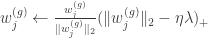
 is a step-size. The authors fixed

 from
from  low dimensional measurements
  in a way that leverages a set of training data
  .
. convex optimization problem
  . In contrast, statistical compressive sensing is a set of methods which recovers
  . This is adapted to a compressive sensing framework of recreating the best
 is the VAE decoding mapping. The optimization is: given some measurements
  , parameterized by encoding and decoding distributions. The objective, derived through information theoretic principles, can be written as:
![\max _ { \phi , \theta } \sum _ { x \in \mathcal { D } } \mathbb { E } _ { Q _ { \phi } ( Y | x ) } \left[ \log p _ { \theta } ( x | y ) \right] \stackrel { \mathrm { def } } { = } \mathcal { L } ( \phi , \theta ; \mathcal { D } )](https://s0.wp.com/latex.php?latex=%5Cmax+_+%7B+%5Cphi+%2C+%5Ctheta+%7D+%5Csum+_+%7B+x+%5Cin+%5Cmathcal+%7B+D+%7D+%7D+%5Cmathbb+%7B+E+%7D+_+%7B+Q+_+%7B+%5Cphi+%7D+%28+Y+%7C+x+%29+%7D+%5Cleft%5B+%5Clog+p+_+%7B+%5Ctheta+%7D+%28+x+%7C+y+%29+%5Cright%5D+%5Cstackrel+%7B+%5Cmathrm+%7B+def+%7D+%7D+%7B+%3D+%7D+%5Cmathcal+%7B+L+%7D+%28+%5Cphi+%2C+%5Ctheta+%3B+%5Cmathcal+%7B+D+%7D+%29&bg=ffffff&fg=333333&s=0&c=20201002)
 is an encoding distribution parameterized like the original sparse coding compression mapping
 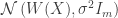 , and
, and  is a variational distribution that decodes
  , which is simply the data itself,
  .
. on MNIST, and use a variety of classification algorithms (k-nearest neighbors, SVMs, etc) on this low-d representation to test classification performance. They find that the UAE linear compression better separates clusters of digits than PCA. It is unclear, however, how this UAE classification performance would compare to linear compression algorithms that are known to work better for classification, such as random projections and ICA. I suspect it will not do as well. Without these comparisons, unclear what use this particular linear mapping provides.
 does a better job at reconstructing
  . That is, the UAE objective written above is the same as the VAE objective minus the KL term. Though a VAE with
 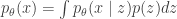 , where
  defines the generative mapping from latents
  , which is also parametrized by a deep neural network (the so-called “encoder”).
![\underset{\theta,\phi}{\text{maximize}}\:\:\mathbb{E}_{q_\phi(z\mid x)}\left[\log p_\theta(x\mid z)\right]-\beta D_{KL}(q_\phi(z\mid x)\Vert\, p(z))](https://s0.wp.com/latex.php?latex=%5Cunderset%7B%5Ctheta%2C%5Cphi%7D%7B%5Ctext%7Bmaximize%7D%7D%5C%3A%5C%3A%5Cmathbb%7BE%7D_%7Bq_%5Cphi%28z%5Cmid+x%29%7D%5Cleft%5B%5Clog+p_%5Ctheta%28x%5Cmid+z%29%5Cright%5D-%5Cbeta+D_%7BKL%7D%28q_%5Cphi%28z%5Cmid+x%29%5CVert%5C%2C+p%28z%29%29&bg=ffffff&fg=333333&s=0&c=20201002)
 . The new hyperparameter
  .
. . Our terminology changes, but the fundamental problem is the same; I made that comparison as obvious as possible in the figure below.
 with a distribution
  , define any statistical mapping
  is just an encoder, and together they induce a joint distribution
  with a marginal
  . The distortion-rate optimization would minimize distortion
  subject to a maximum rate
  , i.e.
![\underset{q_\phi(z\mid x),p(z)}{\text{minimize}}\:\:\mathbb{E}_{p(x,z)}[d(x,z)]\:\:\text{subject to}\:\: I(x,z)\le R](https://s0.wp.com/latex.php?latex=%5Cunderset%7Bq_%5Cphi%28z%5Cmid+x%29%2Cp%28z%29%7D%7B%5Ctext%7Bminimize%7D%7D%5C%3A%5C%3A%5Cmathbb%7BE%7D_%7Bp%28x%2Cz%29%7D%5Bd%28x%2Cz%29%5D%5C%3A%5C%3A%5Ctext%7Bsubject+to%7D%5C%3A%5C%3A+I%28x%2Cz%29%5Cle+R+&bg=ffffff&fg=333333&s=0&c=20201002)
![\Longrightarrow \underset{q_\phi(z\mid x),p(z)}{\text{minimize}}\:\:\mathbb{E}_{p(x,z)}[d(x,z)]-\beta I(x,z)](https://s0.wp.com/latex.php?latex=%5CLongrightarrow+%5Cunderset%7Bq_%5Cphi%28z%5Cmid+x%29%2Cp%28z%29%7D%7B%5Ctext%7Bminimize%7D%7D%5C%3A%5C%3A%5Cmathbb%7BE%7D_%7Bp%28x%2Cz%29%7D%5Bd%28x%2Cz%29%5D-%5Cbeta+I%28x%2Cz%29&bg=ffffff&fg=333333&s=0&c=20201002)


 induced by our choice of encoder
  that makes the optimization more tractable, e.g.
  in the VAE. Our objective can be rewritten as
![\underset{q_\phi(z\mid x),m(z)}{\text{minimize}}\:\:\mathbb{E}_{p(x,z)}[d(x,z)]-\beta\, \mathbb{E}_{x\sim\mathcal{D}}\left[D_{KL}(q_\phi(z\mid x)\Vert\, m(z))\right]](https://s0.wp.com/latex.php?latex=%5Cunderset%7Bq_%5Cphi%28z%5Cmid+x%29%2Cm%28z%29%7D%7B%5Ctext%7Bminimize%7D%7D%5C%3A%5C%3A%5Cmathbb%7BE%7D_%7Bp%28x%2Cz%29%7D%5Bd%28x%2Cz%29%5D-%5Cbeta%5C%2C+%5Cmathbb%7BE%7D_%7Bx%5Csim%5Cmathcal%7BD%7D%7D%5Cleft%5BD_%7BKL%7D%28q_%5Cphi%28z%5Cmid+x%29%5CVert%5C%2C+m%28z%29%29%5Cright%5D&bg=ffffff&fg=333333&s=0&c=20201002)
 . Such a function penalizes representations
  with high probability. A typical distortion-rate problem would fix the distortion function, but we choose to learn this decoder. We can optimize the objective for each
  , and recover the
 ![\underset{q_\phi(z\mid x),p_\theta(x\mid z)}{\text{maximize}}\:\:\mathbb{E}_{q_\phi(z\mid x)}\left[\log p_\theta(x\mid z)\right]-\beta\, D_{KL}(q_\phi(z\mid x)\Vert\, m(z))](https://s0.wp.com/latex.php?latex=%5Cunderset%7Bq_%5Cphi%28z%5Cmid+x%29%2Cp_%5Ctheta%28x%5Cmid+z%29%7D%7B%5Ctext%7Bmaximize%7D%7D%5C%3A%5C%3A%5Cmathbb%7BE%7D_%7Bq_%5Cphi%28z%5Cmid+x%29%7D%5Cleft%5B%5Clog+p_%5Ctheta%28x%5Cmid+z%29%5Cright%5D-%5Cbeta%5C%2C+D_%7BKL%7D%28q_%5Cphi%28z%5Cmid+x%29%5CVert%5C%2C+m%28z%29%29&bg=ffffff&fg=333333&s=0&c=20201002)
 , our optimization prioritizes minimizing the second term (rate) over maximizing the first one (distortion). In this sense, the authors’ argument for large
 , in other words solutions that depend on a good code, not necessarily a good decode. Does eliminating this possibility simply make room to fish out an ad-hoc interpretable representation, or is there a more sophisticated explanation waiting to be found? We’ll see.
 , both centered, where
  is the number of samples), CCA seeks to identify a pair of dimensions
  such that the Pearson’s correlation between the projections
 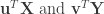 is the largest. In other words, CCA identifies linear combinations of the variables in
  that are the most linearly-related. CCA need not stop there—it can identify pairs of dimensions that monotonically decrease in correlation. In this way, we can ignore the dimensions with the smallest correlations (which likely are spurious). One fun fact about CCA is that any two identified dimensions in
  are uncorrelated:
 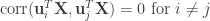 (and the same for
  ). This is different from PCA, whose identified dimensions are both uncorrelated and orthogonal. The uncorrelatedness of CCA dimensions ensures that we do not include dimensions that contain redundant information. (Implementation details: CCA is solved with singular-value decomposition, but be sure to use a regularized form akin to ridge regression—it was unclear if the authors used regularization).
 . The plant is in danger of over-heating and as the operator, you can either keep the plant running or shut it down. Keeping the plant running while the plant’s temperature exceeds a critical threshold
  will cause a nuclear meltdown, incurring a huge loss
  while shutting off the plant for benign temperatures incurs a minor loss
  .
. 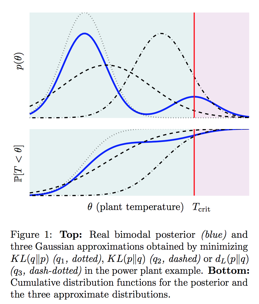
 . Both strategies underestimate the posterior mass for the safety-critical region. Instead, the dash-dotted line, while failing to characterize typical properties of the posterior, results in the same decision as the true posterior by optimizing for task-specific utility. The point is the “best” approximate posterior is subjective, and therefore, we should tailor our inferential resources to find an approximation that is well suited for the decision task at hand.
 , which tells us the utility of taking action
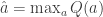
 ![\underset{a}{\arg \min} \text{ } \mathcal{R}(a) = \mathbb{E}_{p(\theta|D)}[U(\theta, a)]](https://s0.wp.com/latex.php?latex=%5Cunderset%7Ba%7D%7B%5Carg+%5Cmin%7D+%5Ctext%7B+%7D+%5Cmathcal%7BR%7D%28a%29+%3D+%5Cmathbb%7BE%7D_%7Bp%28%5Ctheta%7CD%29%7D%5BU%28%5Ctheta%2C+a%29%5D&bg=ffffff&fg=333333&s=0&c=20201002) . Typically, this is computed using a 2-step procedure. First approximate the posterior
. Typically, this is computed using a 2-step procedure. First approximate the posterior  and then minimize the risk under
  . This approach, however, assumes our approximate
