anuththararupasinghe

In this week’s lab meeting, we discussed the paper Neural Network Poisson Models for Behavioural and Neural Spike Train Data, which had been presented by Khajehnejad, Habibollahi, Nock, Arabzadeh, Dayan, and Dezfouli at ICML, 2022. This work aimed to introduce an end-to-end model that explained how the brain represents past and present sensory inputs across areas, and how these representations evolve over time and ultimately lead to behavior. While numerous supervised, reinforcement learning, and unsupervised point process-based methods do exist for examining the relationship between neural activity and behavior, these methods in general have several shortcomings including being insufficient to capture complex neural representations of inputs and actions distributed across different brain regions, not accounting for trial-to-trial variability in behavior and neural recordings, and being sensitive to the choice of bin size of spike counts.

Addressing these limitations, here the authors introduced a novel neural network Poisson process model which models a canonical visual discrimination experiment whereby, on each trial, subjects are presented with a stimulus and have to choose an option (or keep still; i.e. NoGo). The main contributions of this approach can be summarized as follows.

Handles variability between response times across different trials of an experiment by a temporal re-scaling mechanism:
- For each trial $n$ , they considered spikes from unit $u$ until either a response $a_n$ was made at time $r_n$ , or to the end of time window $W$ , whichever had come first, i.e., up to $W_n = \min(W, r_n)$ . The reason for restricting the trial duration accordingly had been to model the neural processes that led to behavioral responses, rather than what happened post-response. To handle the variability of $W_n$ across different trials, they proposed to re-scale the original spike times $t'$ using a trial-specific monotonic function $z_n: [0,W_n] \rightarrow [0,W]$ , $t = z_n(t')$ . Following this transformation, the latent neural intensity function of the inhomogeneous Poisson point process of unit $u$ at trial $n$ and time $\tau$ given by $\lambda^{N}_{u,n}(\tau;\mathbf{h}_n)$ , where $\mathbf{h}_n$ is the stimulus embedding, can be related to the corresponding canonical (trial independent) intensity function $\lambda^{N}_{u}(\tau;\mathbf{h}_n)$ by $\lambda^{N}_{u,n}(t';\mathbf{h}_n) = \lambda^{N}_{u}(z_n(t');\mathbf{h}_n)$ . This facilitates the estimation of a single function $\lambda^{N}_{u}(\tau;\mathbf{h}_n)$ to model the neuronal spiking activities across all trials while preserving details about the variability of response times across different trials. To simplify the subsequent derivations, they assumed this transformation to be linear: $z_n(t') = t' \frac{W}{W_n}$ .
Flexibly learns (without any assumptions on the functional form) the connections between environmental stimuli and neural representations, and between neural representations and behavioral responses:
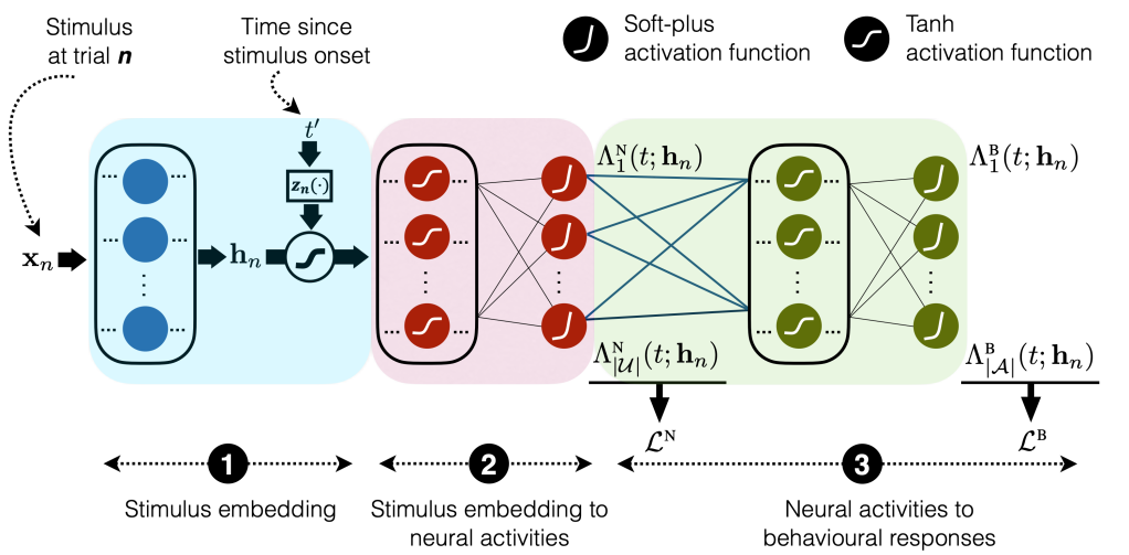
- The following figure shows the model that they proposed to achieve this task, which is a neural network with three main components. The first maps the stimulus $\mathbf{x}_n$ that was presented at trial $n$ through a series of fully connected layers to realize an input embedding denoted by $\mathbf{h}_n$ . The second component takes the embedding $\mathbf{h}_n$ and the spike times $t'$ since the stimulus onset and outputs the modeled activity of each neural region $u$ at time $t$ in the form of the cumulative intensity function $\Lambda^{N}_u(t;\mathbf{h}_n)$ . The neural intensity function $\lambda^{N}_u(t;\mathbf{h}_n)$ is then obtained by differentiating $\Lambda^{N}_u(t;\mathbf{h}_n)$ with respect to $t$ . The motivation for parameterizing the cumulative intensity functions instead of directly parameterizing the neural intensity function had been to obviate the computation of the intractable integral in the point process likelihood. The third component of the model takes the neural cumulative intensity functions and maps them to the behavioral cumulative intensity functions $\Lambda^{B}_a(t;\mathbf{h}_n)$ for making each action $a \in \mathcal{A}$ at each time $t$ since the stimulus onset.
Jointly fits both behavioral and neural data:
- They used the neural loss function $\mathcal{L}^N$ to train all the weights from stimulus to neural cumulative intensity functions (blue and red rectangles in the following figure): $\mathcal{L}^N = \sum_{n=1}^{|\mathcal{N}|}\sum_{u \in \mathcal{U}_n} \mathcal{L}^N_{u.n}$ , where $\mathcal{L}^N_{u.n} = \sum_{i=1}^{|S_{u.n}|} \left[ \log \frac{\partial \Lambda^{N}_u(t= z_n(s_{u.n}^i);\mathbf{h}_n)}{\partial t}\right] - \frac{W_n}{W} \Lambda^{N}_u(W;\mathbf{h}_n)$ , and $s_{u.n}^i$ is the spike time relative to the stimulus onset of the $i^{\sf th}$ spiking event of unit $u$ at trial $n$ . Given these trained neural cumulative intensity functions, then the weights connecting neural outputs to behavioral outputs (green rectangle in the following figure) had been trained using $\mathcal{L}^B = \sum_{a \in \mathcal{A}} \mathcal{L}^B_{a}$ , where $\mathcal{L}^B_{a} = \sum_{n \in \mathcal{N}_a} \log \frac{\partial \Lambda^{B}_a(t= z_n(r_n);\mathbf{h}_n)}{\partial t}- \sum_{n \in \mathcal{N}} \frac{W_n}{W} \Lambda^{B}_a(W;\mathbf{h}_n)$ , and $\mathcal{N}_a$ is the set of trials on which action $a$ was taken before $W$ .
Derives spike count statistics disentangled from chosen temporal bin sizes:
- Since the aforementioned learning process directly uses the spike times as inputs instead of spike counts, this inference is independent of the selection of a time bin for spike count calculations.

Finally, they applied this method to two neural/behavioral datasets concerning visual discrimination tasks: one collected using Neuropixel probes (Steinmetz et al., 2019) from mice, and the other the output of a hierarchical network model with reciprocally connected sensory and integration circuits that modeled behavior in a motion-based task (Wimmer et al., 2015). They showed that this method can link behavioral data with their underlying neural processes and input stimuli in both cases and that it outperforms several existing baseline point process estimators.