dimensionality reduction | Pillow Lab Blog

For this week’s journal club, we covered “Insights on representational similarity in neural networks with canonical correlation” by Morcos, Raghu, and Bengio, NeurIPS, 2018. To date, many different convolutional neural networks (CNNs) have been proposed to tackle the object recognition problem, including Inception (Szegedy et al., 2015), ResNet (He et al., 2016), and VGG (Simonyan and Zisserman, 2015). These networks have vastly different architectures but all achieve high accuracy. How can this be the case? One possibility is that although the architectures vary, the representations (i.e., the way these networks encode information about the objects of natural images) are very similar.

To test this, we first need a metric of similarity. One approach has been “representation similarity analysis” (RSA) (Kriegskorte et al., 2008) which relies on distance matrices to test if two representations are similar. One potential problem with RSA is that some dimensions of the representations may be “noisy” (i.e., dimensions that do not pertain to encoding the input information). For example, during training, some dimensions of the activity of CNN neurons may vary substantially across epochs but are not relevant to encoding object information. These dimensions could mask the signal of relevant dimensions when analyzing a distance matrix.

One way to avoid this is to try to directly identify the relevant dimensions, allowing us to ignore the noisy dimensions. The authors relied on an old but trusted method called canonical correlation analysis (CCA), which was developed way back in the 1930s (Hotelling, 1936)! CCA has been a handy tool in computational neuroscience, relating the activity of neurons across two populations (Semedo et al., 2014) as well as relating population activity to the output of model neurons (Susillo et al., 2015). Newer methods have been developed that are more appropriate for various problems. These include partial least squares (Höskuldsson, 1988), kernel CCA (Hardoon et al., 2004), as well as a method I developed for my own work called distance covariance analysis (DCA) (Cowley et al., 2017). The common thread among all of these methods is that they identify dimensions that encode similar information among two or more datasets.

Overview of CCA. CCA is a close relative to linear regression, but whereas linear regression aims at prediction, CCA focuses on correlation—and thus is most suitable for cases in which the investigator seeks intuition of the data. Given two datasets (e.g., $\mathbf{X} \in \mathcal{R}^{k \times N} \textrm{ and } \mathbf{Y} \in \mathcal{R}^{p \times N}$ , both centered, where $N$ is the number of samples), CCA seeks to identify a pair of dimensions $\mathbf{u} \in \mathcal{R}^k \textrm{ and } \mathbf{v} \in \mathcal{R}^p$ such that the Pearson’s correlation between the projections $\mathbf{u}^T \mathbf{X} \textrm{ and } \mathbf{v}^T \mathbf{Y}$ is the largest. In other words, CCA identifies linear combinations of the variables in $\mathbf{X} \textrm{ and } \mathbf{Y}$ that are the most linearly-related. CCA need not stop there—it can identify pairs of dimensions that monotonically decrease in correlation. In this way, we can ignore the dimensions with the smallest correlations (which likely are spurious). One fun fact about CCA is that any two identified dimensions in $\mathbf{X}$ are uncorrelated: $\textrm{corr}(\mathbf{u}_i^T \mathbf{X}, \mathbf{u}_j^T \mathbf{X}) = 0 \textrm{ for } i \neq j$ (and the same for $\mathbf{v}_i, \mathbf{v}_j$ ). This is different from PCA, whose identified dimensions are both uncorrelated and orthogonal. The uncorrelatedness of CCA dimensions ensures that we do not include dimensions that contain redundant information. (Implementation details: CCA is solved with singular-value decomposition, but be sure to use a regularized form akin to ridge regression—it was unclear if the authors used regularization).

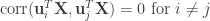
Figure 1. Generalizing networks converge to more similar solutions than memorizing networks.

Onto the results. The authors proposed a distance metric of CCA to uncover some intuitive characteristics about deep neural networks. First, they found that different initializations of generalizing networks (i.e., networks trained on labeled natural images) were more similar than different initializations of memorizing networks (i.e., networks trained on the same dataset with randomly-shuffled labels). This is expected, as natural labels likely put a constraint on generalizing networks. Interestingly, when comparing generalizing and memorizing networks (Fig. 1, yellow line, ‘Inter’), they found that generalizing and memorizing networks were as similar as different memorizing networks trained on the same fixed dataset. This suggests that overfitted networks converge on very different solutions for the same problem. Also interesting was that earlier layers of both generalizing and memorizing networks seem to converge on similar solutions, while the later layers diverged. This suggests that earlier layers rely more on the structure of natural images while the later layers rely more on the structure of the labels. Second, they found that wider networks (i.e., networks with more filters per layer) converge to more similar solutions than those of narrower networks. They argue that this supports the “lottery-ticket” hypothesis that wider networks are more likely to have a sub-network that fits the desired function. Finally, they found that networks trained with different initializations and learning rates on the same problem converge to different groups of solutions. This highlights the need to try different initializations when training neural networks.

This paper left me thinking a lot about representation in the visual cortex of the brain. Does visual cortical population activity have stable and “noisy” dimensions? If we reduced the number of visual cortical neurons per visual cortical area (either via lesion or pharmacological intervention) in a developing animal, would these animals have severe perceptual deficits (i.e., their visual system did not have the right lottery ticket when developing)? Lastly, it seems plausible that humans start out with different initializations of their visual cortices—does that suggest different humans have converged on different solutions to solving visual perception? If so, it suggests that inter-subject variability may be larger than previously thought.

On July 28th, I presented the following paper in lab meeting:

Efficient and direct estimation of a neural subunit model for sensory coding,
Vintch, Zaharia, Movshon, & Simoncelli, NIPS 2012

This paper proposes a new method for characterizing the multi-dimensional stimulus selectivity of sensory neurons. The main idea is that, instead of thinking of neurons as projecting high-dimensional stimuli into an arbitrary low-dimensional feature space (the view underlying characterization methods like STA, STC, iSTAC, GQM, MID, and all their rosy-cheeked cousins), it might be more useful / parsimonious to think of neurons as performing a projection onto convolutional subunits. That is, rather than characterizing stimulus selectivity in terms of a bank of arbitrary linear filters, it might be better to consider a subspace defined by translated copies of a single linear filter.

Continue reading →