
[latexpage]
Last week in lab meeting I discussed a paper from Emily Fox’s group [TFF15], Bayesian Structure Learning for Stationary Time Series.
If you’ve read Carvalho and Scott’s paper on Bayesian inference for graphical models [CS09], then you’ll find [TFF15] a natural extension to [CS09] and reading the latter is surely the best way to get your head wrapped around the former.
From my view [TFF15] makes 2 main contributions:
1) Formulating the graph inference problem in terms of time series by borrowing from [CS09]
2) Formulating the problem in the Fourier domain, making the problem tractable.
On the way to making the problem properly specified, [TFF15] introduced a new conjugate prior on complex normal distributions defined on graphs, the hyper- complex inverse Wishart distribution.
To give you a little background, [CS09] used an algorithm (FINCS, originally developed in [CS08]) for inferring a undirected graph that defines conditional dependence between random variables when
- variables are Gaussian distributed
- observations are independent
- the admissible graphs are “decomposable,” which mean that the graph can be unambiguously described by a bunch of cliques and their intersecting nodes (called “separators”).
Solving the problem in these terms provides some convenient simplifications.
The first simplification, owing to the variables being Gaussian, is a well-known result by Dempster [Demp72],
Suppose 

![[\Sigma]_{ij}^{-1} = 0](https://s0.wp.com/latex.php?latex=%5B%5CSigma%5D_%7Bij%7D%5E%7B-1%7D+%3D+0&bg=ffffff&fg=333333&s=0&c=20201002)

In other words, 


The simplification relies upon the restriction of searching over decomposable graphs on more way than one. Not only does FINCS relyupon this assumption but decomposability provides for a convenient factorization of the prior. Conditioned on the graph 


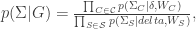
where 
The snag that kept [TFF15] from using [CS09] more or less out of the box is that time series do not have independent observations, except in the trivial case (negating any simplification afforded by assumption (2), in the above list). Thus, the likelihood over times series does not factorize over observations, thereby requiring us to contend with potentially very large covariance matrices. The key insight that [TFF15] made is that moving to the Fourier domain allowed them to make use of the Whittle approximation, which states that Fourier coefficients of stationary times series are asymptotically independent. This is a clever trick that allowed [TFF15] to operate as if the observations 
The complex likelihood required [TFF15] to derive a new hyper-Markov conjugate prior over the covariance matrices (or rather, spectral density matrics 
After specifying the prior over the spectral densities, [TFF15] specify a hyperprior over the graph, which determines the number of edges 


It turns out you can marginalize out both the probability of edges 
You can check out the analysis results for yourselves but I think that they look pretty awesome and make a great argument in favor of their approach.
Now, I’m not an expert on graph theory but I think that the most dubious of the assumptions that [TFF15] inherited from [CS09] is the requirement that all admissible graphs be decomposable. Its not clear to me how (or if) this is a very strong restriction and I’m curious how the algorithm adapts when the model is misspecified. When does it matter? How could this kind of bias influence scientific conclusions drawn from the inferred graphs? I’m also interested in how one might leverage these techniques to infer directed graphs.
If others have intuition about these points then I’m curious to know.
References:
[TFF15] Tank A, Foti NJ, and Fox E. Bayesian Structure Learning for Stationary Time Series. Uncertainty in Artificial Intelligence (UAI), 2015.
[CS09] C. M. Carvalho and J. G. Scott. Objective Bayesian model selection in Gaussian graphical models. Biometrika, 96(3):497?512, 2009
[CS08] C. M. Carvalho and J. G. Scott. Feature-inclusion stochastic search for Gaussian graphical models. J. Computational and Graphical Statistics, 17(4):790-808, 2008
[Demp72] Dempster, A. Covariance selection. Bometics, 28, 157-175
[DaLa93] A. P. Dawid and S. L. Lauritzen. Hyper Markov laws in the statistical analysis of decomposable graphical models. Ann. Statist., 21(3):1272–1317, 1993.

