Today in lab meeting, we continued our discussion of deep unsupervised learning with a tutorial on Normalizing Flows. Similar to VAEs, which we have discussed previously, flow-based models are used to learn a generative distribution, , when this is arbitrarily complex and may, for example, represent a distribution over all natural images. Alternatively, in the context of neuroscience, may represent a distribution over all possible neural population activity vectors. Learning can be useful for missing data imputation, dataset augmentation (deepfakes) or to characterize the data generating process (amongst many other applications).
Flow-based models allow us to efficiently and exactly sample from , as well as to efficiently and exactly evaluate. The workhorse for Normalizing Flows is the Change of Variables formula, which maps a probability distribution over to a simpler probability distribution, such as a multivariate Gaussian distribution, over latent variable space . Assuming a bijective mapping , the Change of Variables formula is
where is the absolute value of the determinant of the Jacobian. This term is necessary so as to ensure probability mass is preserved during the transformation. In order to sample from , a sample from can be converted into a sample from using the inverse transformation:
Flow-models such as NICE, RealNVP, and Glow utilize specific choices for so as to ensure that is both invertible and differentiable (so that both sampling from and evaluating are possible), and so that the calculation of is computationally tractable (and not an operation, where is the dimension of ). In lab meeting, we discussed the Coupling Layers transformation used in the RealNVP model of Dinh et al. (2017):
This is an invertible, differentiable mapping from latent variables , which are sampled from a multivariate normal distribution, to the target distribution. Here ‘‘ denotes elementwise multiplication and and are functions implemented by neural networks. The RealNVP transformation results in a triangular Jacobian with a determinant that can be efficiently evaluated as the product of the terms on the diagonal. We examined the JAX implementation of the RealNVP model provided by Eric Jang in his ICML 2019 tutorial.
As a neural computation lab, we also discussed the potential usefulness of flow-based models in a neuroscience context. Some potential limitations to their usefulness may lie in the fact that they are typically used to model continuous probability distributions; yet in neuroscience, we are often interested in Poisson-like spike distributions. However, recent work on dequantization, which describes how to model discrete pixel intensities with flows, may provide inspiration for how to handle the discreteness of neural data. One other potential limitation to their usefulness related to the fact that the dimensionality of the latent variable in flow-models is equal to that of the observed data. In neuroscience, we are often interested in finding lower-dimensional structure within neural population data; so flow-based models may not be well-suited for this purpose. Regardless of these potential limitations; it is clear that normalizing flows models are powerful and we look forward to continuing to explore their applications in the future.
In lab meeting this week, we discussed Lapses in perceptual judgments reflect exploration by Pisupati*, Chartarifsky-Lynn*, Khanal and Churchland. This paper proposes that, rather than corresponding to inattention (Wichmann and Hill, 2001), motor error, or -greedy exploration as has previously been suggested, lapses (errors on “easy” trials with strong sensory evidence) correspond to uncertainty-guided exploration. In particular, the authors compare empirically-obtained psychometric curves characterizing the performance of rats on a 2AFC task, with predicted psychometric curves from various normative models of lapses. They found that their softmax exploration model explains the empirical data best.
Empirical psychometric curve
Psychometric curves are used to characterize the behavior of animals as a function of the stimulus intensity when performing, for example, 2AFC tasks. They are defined by four parameters:
where is a sigmoidal curve (we will assume the cumulative normal distribution in what follows); determines the decision boundary and is the inverse slope parameter. is the lower asymptote of the curve, while is the upper asymptote. Together, , comprise the asymmetric lapse rates for the “easiest” stimuli (highest intensity stimuli).
While Bayesian ideal observer models have been able to motivate the cumulative normal shape of the psychometric curve (as the authors show in their Methods section), this paper aims to compare different normative models to explain the and parameters of the psychometric curve.
Inattention model
For their inattention model, the authors assume that, with probability , the rat pays attention to the task-relevant stimulus, while, with probability , it ignores the stimulus and instead chooses according to its bias . That is:
or, equivalently, and .
Softmax exploration model
In comparison to the inattention model, which assumes that, when the animal is paying attention to the task-relevant variable, it chooses the action corresponding to the maximum expected action-value, ; the softmax-exploration model assumes that the animal chooses to go right in a 2AFC task according to
where is the inverse temperature parameter and controls the balance between exploration and exploitation and is the difference in the expected value of choosing Right compared to choosing Left (see below). In the limit of , the animal will once again choose its action according to ; while in the low regime, the animal is more exploratory and may choose actions despite them not having the largest expected action values.
In the task they consider, where an animal has to determine if the frequency of an auditory and/or visual cue exceeds a predetermined threshold, the expected action values are , where is the posterior distribution over the category of the stimulus (whether the frequency of the generated auditory and/or visual stimuli are above or below the predetermined threshold) given the animal’s noisy observations of the auditory and visual stimuli, and . is the reward the animal will obtain if it chooses to go Right and is correct. Similarly, .
The authors show that the softmax exploration model corresponds to setting the lapse parameters as
and
Model Comparison
The authors compare the empirically obtained psychometric curves with those predicted by the inattention and exploration models for two experimental paradigms:
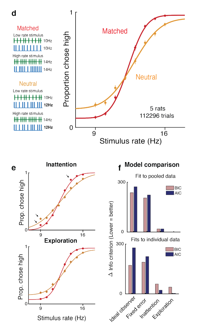
Matched vs Neutral Multisensory stimuli: in this experiment, rats are either presented with auditory and visual stimuli of the same frequency (‘matched’), or with auditory and visual stimuli, where one of the channels has a frequency close to the category threshold, so is, in effect, informationless (‘neutral’). The idea here is that both matched and neutral stimuli have the same ‘bottom-up salience’, so that the parameter is the same for both matched and neutral experiments in the inattention model. By contrast, there is no such restriction for the softmax exploration model, and there is a different exploration parameter for the matched and neutral experiments. The authors find that the psychometric curves corresponding to the softmax model resemble the shape of the empirically obtained curves more closely; and that BIC/AIC are lower for this model.
Reward manipulations: whereas the reward for choosing left or right was previously equal, now the reward for choosing right (when the frequency is above the predetermined threshold) is either increased or decreased. Again, the authors find that the psychometric curves corresponding to the softmax model resemble the shape of the empirically obtained curves more closely; and that BIC/AIC are lower for this model.
(Part of) Figure 3 of Pisupati*, Chartarifsky-Lynn*, Khanal and Churchland. The authors compare the shape of the empirically obtained psychometric curves for the matched and neutral experiments with those obtained by constraining the parameter to be the same for both matched and neutral conditions for the inattention model. In contrast, the parameter is allowed to differ for matched and neutral conditions for the exploration model. The resulting psychometric curves for the exploration model more closely resemble those in (d) and also fit the data better according to BIC/AIC.(Part of) Figure 4 of Pisupati*, Chartarifsky-Lynn*, Khanal and Churchland. Top: The inattention, exploration and fixed error models (the latter of which we did not discuss), make different predictions for the shape of the psychometric curve when the size of the reward on the left and right is modified from equality. Bottom: the empirically determined psychometric curves. Clearly, the empirically determined psychometric curves resemble the curves from the exploration model more closely.
Reflections on this paper
By demonstrating that lapse rates can be manipulated with rewards or by using unisensory compared to multisensory stimuli, this paper highlights that traditional explanations for lapses as being due to a fixed probability of the animal neglecting the task-relevant stimulus; motor-error or greedy exploration are overly-simplistic. The asymmetric effect on left and right lapse rates of modified reward is particularly interesting, as many traditional models of lapses fail to capture this effect. Another contribution that this paper makes is in implicating the posterior striatum and secondary motor cortex as areas which may be involved in determining lapse rates; and better characterizing the role of these areas in lapse behavior than has been done in previous experiments.
This being said, some lab members raised some questions and/or points of concern as we discussed the paper. Some of these points include:
We would have liked to see further justification for keeping the same across the matched and neutral experiments and we question if this is a fair test for the inattention model of lapses. Previous work such as Körding et al. (2007) makes us question whether the animal uses different strategies to solve the task for the matched and neutral experiments. In particular, in the matched experiment, the animal may infer that the auditory and visual stimuli are causally related; whereas in the neutral experiment, the animal may detect the two stimuli as being unrelated. If this is true, then it seems strange to assume that and for the inattention model should be the same for the matched and neutral experiments.
When there are equal rewards for left and right stimuli, is there only a single free parameter determining the lapse rates in the exploration model (namely )? If so, how do the authors allow for asymmetric left and right lapse rates for the exploration model curves of Figure 3e (that is, the upper and lower asymptotes look different for both the matched and neutral curves despite equal left and right reward, yet the exploration model seems able to handle this – how does the model do this?).
How could uncertainty be calculated by the rat? Can the empirically determined values of be predicted from, for example, the number of times that the animal has seen the stimulus in the past? And what were some typical values for the parameter when the exploration model was fit with data? How exploratory were the rats for the different experimental paradigms considered in this paper?
In lab meeting this week, we read Deep Neural Networks as Gaussian Processes by Lee, Bahri, Novak, Schoenholz, Pennington and Sohl-Dickstein, and which appeared at ICLR 2018. The paper extends a result derived by Neal (1994); and the authors show that there is a correspondence between deep neural networks and Gaussian processes. After coming up with an efficient method to evaluate the associated kernel, the authors compared the performance of their Gaussian process model with finite width neural networks (trained with SGD) on an image classification task (MNIST, CIFAR-10). They found that the performance of the finite width networks approached that of the Gaussian process performance as the width increased, and that the uncertainty captured by the Gaussian process correlated with mean squared prediction error. Overall, this paper hints at new connections between Gaussian processes and neural networks; and it remains to be seen whether future work can harness this connection in order to extend Gaussian process inference to larger datasets, or to endow neural networks with the ability to capture uncertainty. We look forward to following progress in this field.
Single Layer Neural Networks as Gaussian Processes – Neal 1994
Let us consider a neural network with a single hidden layer. We can write the ith output of the network, , as
where is the post-activation of the jth neuron in the hidden layer; is some nonlinearity, and is the kth input to the network.
If we now assume that the weights for each layer in the network are sampled i.i.d. from a Gaussian distribution: , ; and that the biases are similarly sampled: and ; then it is possible to show that, in the limit of , , for a kernel which depends on the nonlinearity. In particular, this follows from application of the Central Limit Theorem: for a fixed input to the network , as where (which is the same for all ).
We can now apply a similar argument to the above in order to examine the distribution of ith output of the network for a collection of inputs: that is we can examine the joint distribution of . Application of the Multidimensional Central Limit Theorem tells us that, in the limit of ,
,
where and and .
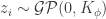
Since we get a joint distribution of this form for any finite collection of inputs to the network, we can write that , as this is the very definition of a Gaussian process.
This result was shown in Neal (1994); and the precise form of the kernel was derived for the error function (a form of sigmoidal activation function) and Gaussian nonlinearities in Williams (1997).
Deep Neural Networks as Gaussian Processes
Lee et al. use similar arguments to those presented in Neal (1994) to show that the th output of the th layer of a network with a Gaussian prior over all of the weights and biases is a sample from a Gaussian process in the limit of . They use an inductive argument of the form: suppose that (the jth output of the th layer of the network is sampled from a Gaussian process). Then:
is Gaussian distributed as and any finite collection of will have a joint multivariate Gaussian distribution, i.e., where
.
If we assume a base kernel of the form , these recurrence relations can be solved in analytic form for the ReLU nonlinearity (as was demonstrated in Cho and Saul (2009)), and they can be solved numerically for other nonlinearities (and Lee et al., give a method for finding the numerical solution efficiently).
Comparison: Gaussian Processes and Finite Width Neural Networks
Lee et al. went on to compare predictions made via Gaussian process regression with the kernels obtained by solving the above recurrence relations (for nonlinearities ReLU and tanh), with the predictions obtained from finite width neural networks trained with SGD. The task was classification (reformulated as a regression problem) of MNIST digits and CIFAR-10 images. Overall, they found that their “NNGP” often outperformed finite width neural networks with the same number of layers for this task; and they also found that the performance of the finite width networks often approached that of the NNGP as the width of these networks was increased:
Figure 1 of Lee et al. The authors compare the performance of their NNGP to finite width neural networks of the same depth and find that, for many tasks, the NNGP outperforms the finite width networks and that the performance of the finite width networks approaches that of the NNGP as the width is increased.


 -greedy exploration as has previously been suggested, lapses (errors on “easy” trials with strong sensory evidence) correspond to uncertainty-guided exploration. In particular, the authors compare empirically-obtained psychometric curves characterizing the performance of rats on a 2AFC task, with predicted psychometric curves from various normative models of lapses. They found that their softmax exploration model explains the empirical data best.
 is a sigmoidal curve (we will assume the cumulative normal distribution in what follows);
  determines the decision boundary and
  is the inverse slope parameter.
  is the lower asymptote of the curve, while
  is the upper asymptote. Together,
  , comprise the asymmetric lapse rates for the “easiest” stimuli (highest intensity stimuli).
  parameters of the psychometric curve.
  , the rat pays attention to the task-relevant stimulus, while, with probability
  , it ignores the stimulus and instead chooses according to its bias
  . That is:
 and
and  .
. ; the softmax-exploration model assumes that the animal chooses to go right in a 2AFC task according to
 is the inverse temperature parameter and controls the balance between exploration and exploitation and
  is the difference in the expected value of choosing Right compared to choosing Left (see below). In the limit of
  , the animal will once again choose its action according to
  , where
  is the posterior distribution over the category of the stimulus (whether the frequency of the generated auditory and/or visual stimuli are above or below the predetermined threshold) given the animal’s noisy observations of the auditory and visual stimuli,
  and
and  .
.  is the reward the animal will obtain if it chooses to go Right and is correct. Similarly,
  .
.  and
and 

 greedy exploration are overly-simplistic. The asymmetric effect on left and right lapse rates of modified reward is particularly interesting, as many traditional models of lapses fail to capture this effect. Another contribution that this paper makes is in implicating the posterior striatum and secondary motor cortex as areas which may be involved in determining lapse rates; and better characterizing the role of these areas in lapse behavior than has been done in previous experiments.
 , as
, as 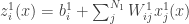
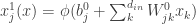 is the post-activation of the jth neuron in the hidden layer;
  is some nonlinearity, and
  is the kth input to the network.
  ,
, 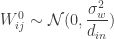 ; and that the biases are similarly sampled:
  and
and  ; then it is possible to show that, in the limit of
  ,
,  , for a kernel
  which depends on the nonlinearity. In particular, this follows from application of the Central Limit Theorem: for a fixed input to the network
  ,
,  as
as ![V_{\phi}(x^{1}(\vec{x})) \equiv \mathbb{E}[(x^{1}_{i}(\vec{x}))^{2}]](https://s0.wp.com/latex.php?latex=V_%7B%5Cphi%7D%28x%5E%7B1%7D%28%5Cvec%7Bx%7D%29%29+%5Cequiv+%5Cmathbb%7BE%7D%5B%28x%5E%7B1%7D_%7Bi%7D%28%5Cvec%7Bx%7D%29%29%5E%7B2%7D%5D&bg=ffffff&fg=333333&s=0&c=20201002) (which is the same for all
(which is the same for all  ).
).  . Application of the Multidimensional Central Limit Theorem tells us that, in the limit of
  ,
,  and
and  and
and ![C_{\phi}(\vec{x}, \vec{x'}) \equiv \mathbb{E}[x_{i}^{1}(\vec{x})x_{i}^{1}(\vec{x}')]](https://s0.wp.com/latex.php?latex=C_%7B%5Cphi%7D%28%5Cvec%7Bx%7D%2C+%5Cvec%7Bx%27%7D%29+%5Cequiv+%5Cmathbb%7BE%7D%5Bx_%7Bi%7D%5E%7B1%7D%28%5Cvec%7Bx%7D%29x_%7Bi%7D%5E%7B1%7D%28%5Cvec%7Bx%7D%27%29%5D&bg=ffffff&fg=333333&s=0&c=20201002) .
.  , as this is the very definition of a Gaussian process.
 th layer of a network with a Gaussian prior over all of the weights and biases is a sample from a Gaussian process in the limit of
  . They use an inductive argument of the form: suppose that
  (the jth output of the
  th layer of the network is sampled from a Gaussian process). Then:
 will have a joint multivariate Gaussian distribution, i.e.,
  where
where ![K_{\phi}^{l}(\vec{x}, \vec{x'}) \equiv \mathbb{E}[z_{i}^{l}(\vec{x})z_{i}^{l}(\vec{x'})] = \sigma_{b}^{2} + \sigma_{w}^{2} \mathbb{E}_{z_{i}^{l-1}\sim \mathcal{GP}(0, K_{\phi}^{l-1})}[\phi(z_{i}^{l-1}(\vec{x})) \phi(z_{i}^{l-1}(\vec{x'}))]](https://s0.wp.com/latex.php?latex=K_%7B%5Cphi%7D%5E%7Bl%7D%28%5Cvec%7Bx%7D%2C+%5Cvec%7Bx%27%7D%29+%5Cequiv+%5Cmathbb%7BE%7D%5Bz_%7Bi%7D%5E%7Bl%7D%28%5Cvec%7Bx%7D%29z_%7Bi%7D%5E%7Bl%7D%28%5Cvec%7Bx%27%7D%29%5D+%3D+%5Csigma_%7Bb%7D%5E%7B2%7D+%2B+%5Csigma_%7Bw%7D%5E%7B2%7D+%5Cmathbb%7BE%7D_%7Bz_%7Bi%7D%5E%7Bl-1%7D%5Csim+%5Cmathcal%7BGP%7D%280%2C+K_%7B%5Cphi%7D%5E%7Bl-1%7D%29%7D%5B%5Cphi%28z_%7Bi%7D%5E%7Bl-1%7D%28%5Cvec%7Bx%7D%29%29+%5Cphi%28z_%7Bi%7D%5E%7Bl-1%7D%28%5Cvec%7Bx%27%7D%29%29%5D&bg=ffffff&fg=333333&s=0&c=20201002) .
. , these recurrence relations can be solved in analytic form for the ReLU nonlinearity (as was demonstrated in
