Step-by-step procedure for choosing a learning rate (and other optimization hyperparameters)

I’ve been using deep neural networks (DNNs) in my research. DNNs, as is often preached, are powerful models, capable of mapping almost any function. However, after the sermon is over, someone starting to train a DNN in the wild can quickly be overwhelmed by the many subtle technical details involved. The architecture, regularization techniques, and optimization are all inter-related, and these relationships change for different datasets.

My first steps in training a DNN primarily focused on architecture—do I have enough layers and filters for my problem? The optimization—stochastic gradient descent (SGD) with all of its hyperparameters (learning rate, momentum, …) and variants—was an afterthought, and I chose hyperparameters that seemed reasonable. Still, a nagging question persisted in the back of my mind: What if different hyperparameters led to even better performance? It was an obvious case of fear-of-missing-out (FOMO).

Grid search (aka brute force) and black-box optimization techniques should be last resorts.

Due to FOMO, I began to more properly choose my hyperparameters by using a grid search (e.g., random search). This takes a lot of time. For each tweak of the architecture, I would need to rerun the entire grid search. For each grid search, out popped a solution and nothing else—no intuition about my problem, no understanding about the tradeoffs of the hyperparameters, and no clear way to check my code for bugs (except evaluating performance). The same can be said for black-box optimization techniques—which are fancier versions of grid search. I felt ashamed each grid search I ran because it’s brainless. It encourages me not to think about my data, model, or the bridge between the two: optimization.

Let’s use our intuition about optimization to help guide our choice of hyperparameters.

Optimization is not a black-box method. In fact, gradient descent is one of the most intuitive concepts in math: You are a hiker on top of a mountain, and you need to get down. What direction and how far do you move? Inspired by this, I started reading about other ways to choose optimization hyperparameters. I came up with a step-by-step procedure that I now follow for every problem. It’s largely inspired by Smith 2018 and Jordan 2018.

This procedure outputs:
1) reasonable values for the hyperparameters,
2) intuition about the problem, and
3) red flags if there are bugs in your code.
The procedure takes a couple of training runs (fast!).

[Note: This procedure is great for researchers who want to get a model up and running. Grid/black-box search is more appropriate for architecture searches and when you really care about gaining 1% in accuracy.]

Step-by-step procedure:

Here’s the full procedure. I’ll discuss each step individually.

1. Compute initial line search.
2. Increase learning rate.
3. Increase momentum.
4. Check if learning rate decay helps.
5. Check if a cyclical learning rate helps.
6. (optional) Check your other favorite SGD variants.
7. Compute final line search, for closure.

The procedure is general for any architecture and problem. For an example problem, I run the procedure on a small (3-layer) convolutional neural network to predict the responses of visual cortical neurons from image features (see Cowley and Pillow, 2020). I report accuracy on heldout data, as we want to make sure our optimized solution generalizes. The description of each step is short for ease of mind; I assume you are familiar with optimization and SGD (if you aren’t, check out the Convex Optimization book).

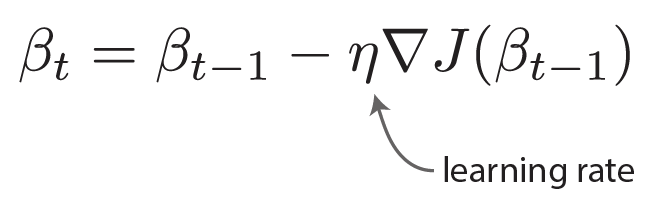
For a quick review, here is the equation for gradient descent:

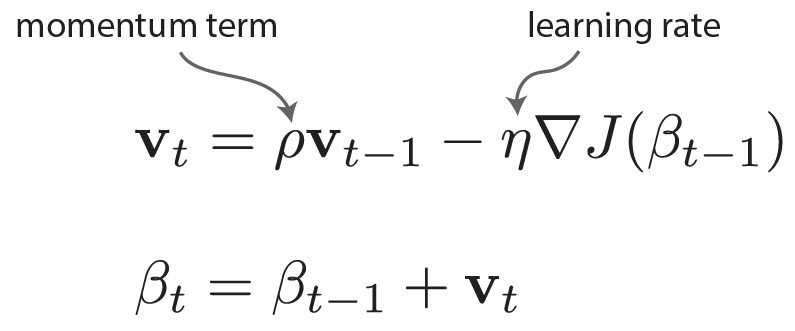
And here are the equations for gradient descent with momentum:

Step 1: Compute initial line search.

• Choose a direction in weight space (found either by training on a small amount of data or choosing weights randomly). 
• Perform a line search by taking small steps (linear increments) along that direction, plotting accuracy for each step.

• How nonconvex/complicated is your accuracy landscape? Here, I have a nonconvex problem with a meandering slope and a sharp ridge with a cliff.
  → Choosing a large learning rate may mean I fall off the cliff!

Step 2: Increase learning rate.

• Start with an epsilon-small learning rate. Then, increase the learning rate for each consecutive training epoch.

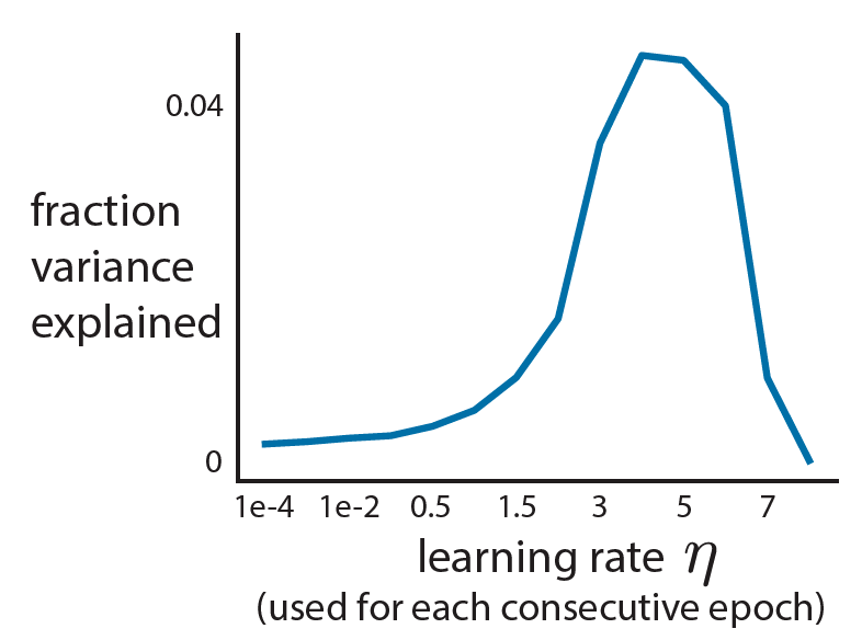
• Small learning rates lead to small increases in accuracy.
  → You’ve barely moved in weight space.
• Large learning rates lead to large decreases in accuracy.
  → You’re moving too far, and you’ve jumped off the cliff!
• Just right learning rates are where the accuracy increases steadily.
• Here, we choose a learning rate of 1.5.

Step 3: Increase momentum.

• Train for N epochs with the chosen learning rate.
• Similar to Step 2, start with a small momentum and increase it each training epoch.

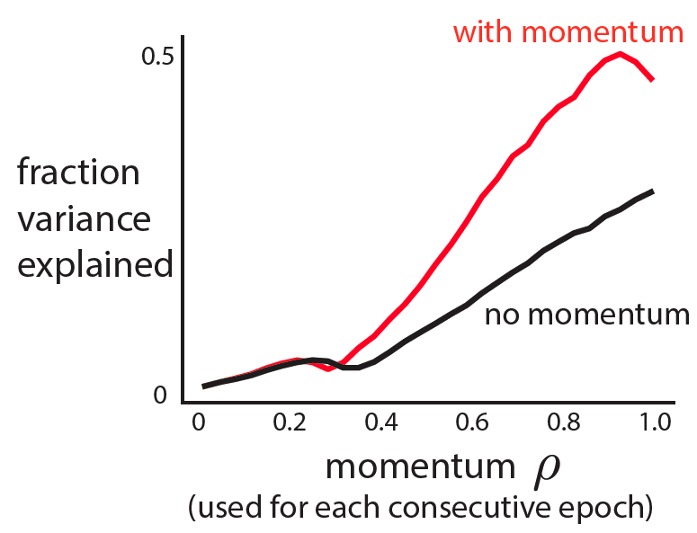
• A small momentum yields only a small increase in accuracy.
  A large momentum sees a drop in accuracy. 
• Choose a momentum in the sweet spot—where accuracy is steadily increasing.
• Here, we choose a momentum of 0.7.

• Using the chosen learning rate and momentum, train for N epochs. Confirm that momentum improves performance.

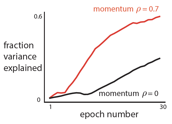
• Thoughts: Momentum does help in this case (red above black).

Step 4: Check if learning rate decay helps.

• Train model until convergence (might be longer than N epochs). 
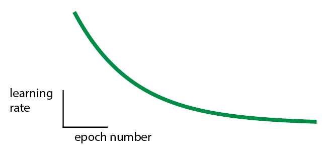
• Use a schedule for learning rate decay. The idea is that as you get closer to an optimum, you should make smaller steps (i.e., decay) to prevent yourself from jumping passed the optimum. Lots of choices here.
• My schedule is a power decay:
  Let M be the epoch number where performance plateaus/falls off.
  Then alpha = (⅔)^(1/M).
  

• Train model with learning rate decay. Confirm learning rate decay is needed.

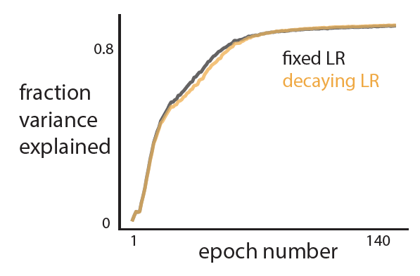
• Thoughts: Learning rate decay is not really helpful for my problem. So I won’t use it.

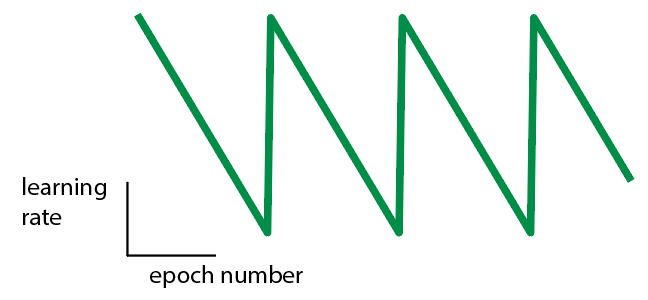
Step 5: Check if a cyclical learning rate helps.

• Use a cyclical learning rate. The idea is that you may want to explore different optima, so we need a way to push ourselves far from the current optimum. 
  
  Here’s one option:
  • Choose the upper learning rate bound as 2 * chosen learning rate.
  • Choose the lower learning rate bound as ½ * chosen learning rate.
  • Start the learning rate at the upper bound then shrink to the lower bound after M epochs (where M is chosen from Step 4). Then, switch back to the largest learning rate:

• Train model with a cyclical learning rate. Confirm that a cyclical learning rate is needed.

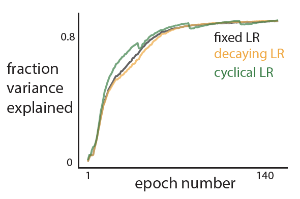
• Thoughts: A cyclical learning rate does train faster, but not substantially. So I won’t use it.

Step 6: (optional) Check your other favorite SGD variants.

• Likely everyone has their favorite SGD variant. Try it here!
  Note: Don’t use the hyperparameters chosen above for some SGD variants, like Adam (which usually assumes a very small initial learning rate). Instead, you may need to repeat some steps to find the variant’s hyperparameters.
• I ran Adam on the same dataset, choosing a learning rate of 1-e2 (much smaller than the learning rate of 1.5 chosen in Step 1!).

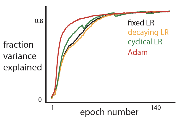
• Adam does well in the beginning, likely because it adapts its learning rate and can get away with a large learning rate for the earlier epochs.
• I’ve found that Adam doesn’t always work well. This is especially true when training a DNN to predict behavior of different subjects—each subject’s behavior (e.g., velocity) may have a different variance. This is why we check!

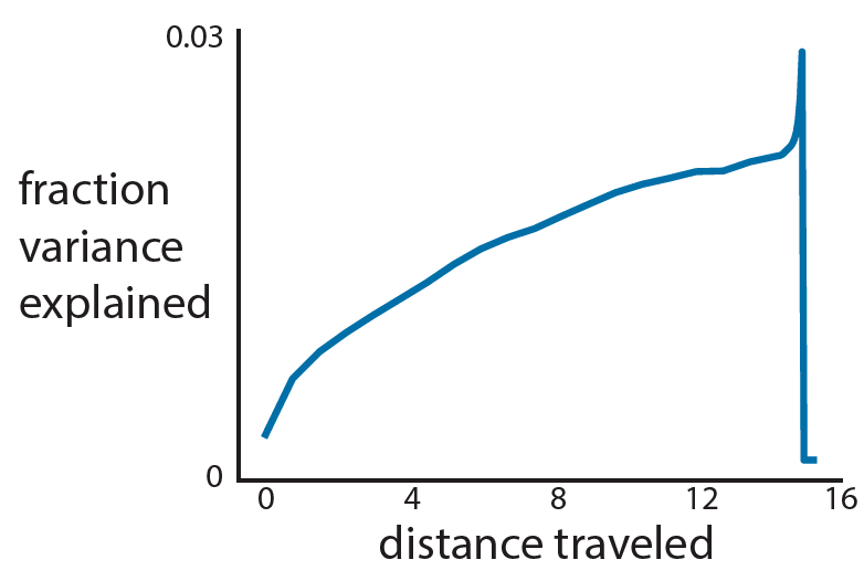
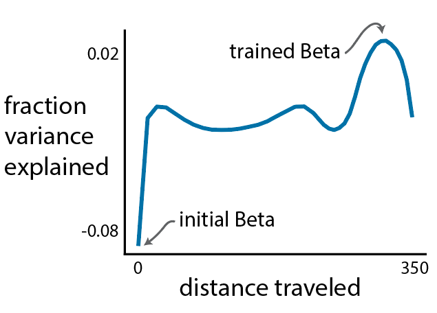
Step 7: Compute final line search, for closure.

• This is my favorite step. It’s the exact same as Step 1, except we now compute a line search in weight space along a line between the initial, untrained weight vector and the final, trained weight vector.

• Thoughts: This looks very similar to Step 1. The optimization first finds the ridge and then moves along this ridge.
• In this example, there doesn’t seem to be multiple local minima. But this is not always the case!  Here’s a final line search from one of my other research projects:

Final thoughts

You can see why I like this procedure so much. It takes about an afternoon to run, and I get some interesting plots to look at and think about. The procedure outputs a nice set of hyperparameters, some intuition about the optimization problem we face, and gives me peace of mind that I shouldn’t keep twiddling hyperparameters and preventing my FOMO.

It would be great to have a gallery of observed final line searches (Step 7), just to see the variety of loss landscapes out there. In the meantime, you can check out these artistic renderings of loss landscapes: losslandscape.com. 

Attention is all you need. (aka the Transformer network)

No matter how we frame it, in the end, studying the brain is equivalent to trying to predict one sequence from another sequence. We want to predict complicated movements from neural activity. We want to predict neural activity from time-varying stimuli. We even want to predict neural activity in one brain area from neural activity in another area. Thus, as computational neuroscientists, we should be intimately familiar with new machine learning techniques that allow us to better relate one sequence to another.

One sequence-to-sequence problem receiving a lot of interest in machine learning is “translation”—converting a sentence in one language (e.g., English) to another (e.g., Polish). The main challenge is getting context correct. For example, consider “bark” for the following sentences: “The bark is loud.” and “The bark is brown.” In Polish, bark would be “szczekanie” and “kora,” respectively, based on context. Machine learning folks have devised some ingenious architectures to tackle this problem. In this post, I’ll talk about one architecture that is unexpected but seems to work quite well: Transformer networks. This architecture was proposed in “Attention is all you need.” by Vaswani, Shazeer, Parmar, Uszkoreit, Jones, Gomez, Kaiser, Polosukhin, NIPS 2017.

High-level intuition

The Transformer network relies on an encoding-decoding approach. The idea is to “encode” the input sequence into a latent representation (i.e., an embedding) that is easier to work with. This embedding (typically a vector of abstract variables) is then “decoded” into an output sequence (e.g., another language). Our problem, then, is to design a “useful” embedding for translation, and build an architecture that can express it.

What properties do we want our embedding to have? One property is a measure of similarity— “tomato” is more similar to “blueberry” than to “chair.” An embedding with this property has been solved with word2vec. Another important property is context—is “tomato” the subject? direct object? is it modified by “tasty” or “rotten”? It turns out we can incorporate context by adding embeddings together. For example, let embeddings e1=”tomato” and e2=”tasty”. Then
e3 = e1 + e2 corresponds to an embedding of a “tasty tomato”. We can keep tacking on more context (e.g., e4 = “subject of sentence”, e5 = “the”, e6 = “belongs to Tom”, etc.). With this embedding property, if we come across an ambiguous word like “it”, we simply find the word that “it” refers to, and add that word to the embedding!

Architecture: Stacked attention layers

The authors came up with a way to efficiently search for context and add that context to the embedding. They use “attention”—in the general sense of the word, not based on neuroscience—as a way to find distant relationships between words. Figure 1 is a stylized version of this computation. The idea is, given a word, compare this word with all other words in the sentence for a specific context. For example, if the word is “sees”, attention will try to find “who sees?” and “sees what?” If attention finds answers to its context questions, these answers will be incorporated into the embedding via a linear combination. If attention does not receive answers, no harm is done—attention will simply pass on the unmodified word embedding (i.e., weights for the other words will be zero).

Figure 1: The attention mechanism. (this is my first time making gifs—sorry for the blurriness!)

One can imagine that having one level of attention may not be the best way to extract the structure of natural language. Just like we learned in sixth grade, sentences have hierarchical structure (did you also have to draw those syntax trees?). So, we should stack levels of attention. The lower levels correspond to easy questions (“Is there an adjective to this noun?”) that likely involve only two or three words of the input sequence. The deeper levels correspond to more nuanced questions (“What is the direct object of this sentence?”) that span most if not all of the input sequence. To achieve this, the authors stacked layers of attention on top of each other. To decode, they basically reverse the process. Figure 2 is an illustration of this process. 

Figure 2: Attention blocks form an encoder stack, which feeds into a decoder stack.

The authors claim this approach minimizes the distance of relating one position in a sequence to another. This is because attention looks at all pairwise interactions, while other architectures (such as recurrent neural networks) sequentially look at the input sequence (making it difficult to compare the first word to the last word). The primary point of confusion while reading the paper was how input sequences were fed into the network (hopefully Fig. 2 clarifies this—each word embedding is transformed in parallel to other word embeddings. If you input N words, each encoder will output N embeddings). This architecture produced state-of-the-art results, and has since been used in many different natural language processing tasks. It also uses many bells and whistles (residual blocks, layer normalization, …)—it will be interesting to see future work argue which components are the most important for this architecture.

Getting back to the neuroscience

As computational neuroscientists, we should take advantage of these architectures (which have been designed and trained with the aid of GPU armies), and use them to help solve our own problems. One aspect of this work (and in natural language processing in general) is the idea of adding two embedding vectors to form a more “context-relevant” embedding. This is missing from our current latent variable models. More importantly, it may be a way in which the brain also encodes context. I also think this type of attention computation will be useful when we are trying to predict sequences of natural behavior, where we cannot make use of task structure (e.g., a delay period, stimulus onset, etc.). Experimentalists are now collecting massive datasets of natural behavior—a perfect opportunity to see how this attention computation holds up!

The Lottery Ticket Hypothesis

Deep learning is black magic. For some reason, a neural network with millions of parameters is not cursed to overfit. Somewhere, either in the architecture or the training or the weights themselves, exists a magic that allows deep neural networks to generalize.  We are now only beginning to understand why this is.  As in most cases in science, a good starting place is to observe a paradox about the system, suggest a hypothesis to explain the paradox, and then test, test, test.

The Paradox: This week we discussed “The lottery ticket hypothesis: Finding sparse, trainable neural networks” by Frankle and Carbin, ICML, 2019. Recent studies have shown that a deep neural network can be pruned down to as little as 10% of the size of the original network with no loss in test prediction. This leads to a paradox: Training the small, pruned network (randomly initialized) leads to worse test prediction than training a large network and then pruning it. This is heresy to the ML doctrine of “Thou shalt start simple, and then go complex.” What is going on?

The Hypothesis: This paradox suggests that the initialization of the weights of the pruned network matters.  This leads to the Lottery Ticket Hypothesis:

The Lottery Ticket Hypothesis: “dense, randomly-initialized, feed-forward networks contain subnetworks (i.e., winning tickets) that—when trained in isolation—reach test prediction comparable to the original network in a similar number of iterations.” 

These “winning tickets” start out with an initialization that make training particularly effective.  If the winning tickets were re-initialized randomly, they would no longer be winning tickets—training would not reach the same level of test prediction. This may explain why deep and wide networks tend to perform better than shallow, narrow networks—> the deeper, wider networks have more chances of having the winning ticket. It also suggests that training a neural network is akin to stochastic gradient descent seeking out these winning tickets.

The Test, Test, Test: To find the winning ticket, the authors employ iterative pruning. They start with a large neural network, train it a bit, set the smallest-magnitude weights to zero (these weights are no longer trainable), rewind the trainable parameters to their original initialized values, and train again. This is repeated until pruning drastically hurts test prediction. They find that these winning tickets can be as sparse as 3.7% of the original network’s size while having the same if not higher test prediction (Figure 1, solid lines). Interestingly, if they randomly re-initialize the weights of these pruned networks, test prediction decreases considerably  (Figure 1, dashed lines, ‘reinit’). Thus, we have a way to identify winning tickets, these winning tickets are a measly fraction of the size of the original network, and their original initialization is crucial to train them.  The authors do a thorough job of confirming the robustness of this effect (45 figures in all). However, they did not investigate the properties of the subnetworks (e.g., did pruning happen most in the deeper layers?).

Figure 1. Winning tickets (subnetworks of large, original network) still maintain high test prediction (solid lines; 7.1% has higher accuracy than 100%). If these winning tickets were randomly initialized then trained (reinit), test prediction suffers (dashed lines below solid lines at 7.1%). Results include three convolutional neural networks at different depths trained and tested on the CIFAR10 image dataset. Figure reproduced from Frankle and Carbin, 2019.

One question I had remaining is if these winning tickets were necessary or sufficient to train the large network.  One analysis that could get at this question is the following. First, identify a winning ticket, and then re-initialize its weights in the original, large network. This ensures that this subnetwork is no longer is a winning ticket. Keep repeating this process.  After removing winning tickets, does the large network fail to train? How many winning tickets does the large network have?  Will the large network always have a winning ticket?  We could also do the reverse of this: For a large network, keep initializing subnetworks that are winning tickets.  Is it the case that with more winning tickets, the network trains faster with higher test prediction?

Implications for deep learning: There are several implications for deep learning. 1. Finding out what is special about the initializations of these winning tickets may help us improve initialization strategies. 2. We may be able to improve optimization techniques by better guiding stochastic gradient descent to find and train the winning ticket as fast as possible. 3. New theory that focuses on subnetworks may lead to more insight into deep learning.  4. These winning tickets may be helpful for solving other tasks (i.e., transfer learning). There have already been some follow up studies about these issues and re-examining the lottery ticket hypothesis:  Liu et al., 2019, Crowley et al., 2019, Frankle et al., 2019, Zhou et al, 2019.

Does the brain have winning tickets? I had one recurring thought while reading this paper: I know brains prune synaptic connections substantially during development—could the brain also consist of whittled-down winning tickets? After some searching, I realized that it is largely unknown the amount of pruning that occurs or when certain pruning happens.  What would be some tell-tale signs of winning tickets?  First, substantial pruning should occur (and likely does…perhaps as much as 50%). Second, randomly initializing a developing circuit should lead to a drop in performance after the same amount of training as a control subject (not sure if we can randomly set synaptic weights yet). Third, what would happen if we could prune small-magnitude synaptic connections ourselves during development? Could the brain recover? These tests could first be carried out in insects, where we have gene lines, optogenetics, whole-brain recordings, and well-labeled cell types. 

Insights on representational similarity in neural networks with canonical correlation

For this week’s journal club, we covered “Insights on representational similarity in neural networks with canonical correlation” by Morcos, Raghu, and Bengio, NeurIPS, 2018.  To date, many different convolutional neural networks (CNNs) have been proposed to tackle the object recognition problem, including Inception (Szegedy et al., 2015), ResNet (He et al., 2016), and VGG (Simonyan and Zisserman, 2015). These networks have vastly different architectures but all achieve high accuracy. How can this be the case? One possibility is that although the architectures vary, the representations (i.e., the way these networks encode information about the objects of natural images) are very similar. 

To test this, we first need a metric of similarity. One approach has been “representation similarity analysis” (RSA) (Kriegskorte et al., 2008) which relies on distance matrices to test if two representations are similar. One potential problem with RSA is that some dimensions of the representations may be “noisy” (i.e., dimensions that do not pertain to encoding the input information). For example, during training, some dimensions of the activity of CNN neurons may vary substantially across epochs but are not relevant to encoding object information. These dimensions could mask the signal of relevant dimensions when analyzing a distance matrix. 

One way to avoid this is to try to directly identify the relevant dimensions, allowing us to ignore the noisy dimensions. The authors relied on an old but trusted method called canonical correlation analysis (CCA), which was developed way back in the 1930s (Hotelling, 1936)! CCA has been a handy tool in computational neuroscience, relating the activity of neurons across two populations (Semedo et al., 2014) as well as relating population activity to the output of model neurons (Susillo et al., 2015). Newer methods have been developed that are more appropriate for various problems. These include partial least squares (Höskuldsson, 1988), kernel CCA (Hardoon et al., 2004), as well as a method I developed for my own work called distance covariance analysis (DCA) (Cowley et al., 2017).  The common thread among all of these methods is that they identify dimensions that encode similar information among two or more datasets.

Overview of CCA. CCA is a close relative to linear regression, but whereas linear regression aims at prediction, CCA focuses on correlation—and thus is most suitable for cases in which the investigator seeks intuition of the data.  Given two datasets (e.g., , both centered, where is the number of samples), CCA seeks to identify a pair of dimensions such that the Pearson’s correlation between the projections is the largest. In other words, CCA identifies linear combinations of the variables in that are the most linearly-related. CCA need not stop there—it can identify pairs of dimensions that monotonically decrease in correlation. In this way, we can ignore the dimensions with the smallest correlations (which likely are spurious). One fun fact about CCA is that any two identified dimensions in are uncorrelated: (and the same for ). This is different from PCA, whose identified dimensions are both uncorrelated and orthogonal.  The uncorrelatedness of CCA dimensions ensures that we do not include dimensions that contain redundant information. (Implementation details: CCA is solved with singular-value decomposition, but be sure to use a regularized form akin to ridge regression—it was unclear if the authors used regularization). 

Figure 1. Generalizing networks converge to more similar solutions than memorizing networks.

Onto the results. The authors proposed a distance metric of CCA to uncover some intuitive characteristics about deep neural networks. First, they found that different initializations of generalizing networks (i.e., networks trained on labeled natural images) were more similar than different initializations of memorizing networks (i.e., networks trained on the same dataset with randomly-shuffled labels). This is expected, as natural labels likely put a constraint on generalizing networks. Interestingly, when comparing generalizing and memorizing networks (Fig. 1, yellow line, ‘Inter’), they found that generalizing and memorizing networks were as similar as different memorizing networks trained on the same fixed dataset. This suggests that overfitted networks converge on very different solutions for the same problem. Also interesting was that earlier layers of both generalizing and memorizing networks seem to converge on similar solutions, while the later layers diverged. This suggests that earlier layers rely more on the structure of natural images while the later layers rely more on the structure of the labels. Second, they found that wider networks (i.e., networks with more filters per layer) converge to more similar solutions than those of narrower networks.  They argue that this supports the “lottery-ticket” hypothesis that wider networks are more likely to have a sub-network that fits the desired function.  Finally, they found that networks trained with different initializations and learning rates on the same problem converge to different groups of solutions. This highlights the need to try different initializations when training neural networks.

This paper left me thinking a lot about representation in the visual cortex of the brain. Does visual cortical population activity have stable and “noisy” dimensions?  If we reduced the number of visual cortical neurons per visual cortical area (either via lesion or pharmacological intervention) in a developing animal, would these animals have severe perceptual deficits (i.e., their visual system did not have the right lottery ticket when developing)?  Lastly, it seems plausible that humans start out with different initializations of their visual cortices—does that suggest different humans have converged on different solutions to solving visual perception?  If so, it suggests that inter-subject variability may be larger than previously thought.