Deep kernel with recurrent structure

This week in lab meeting, we discussed the following work:

Learning Scalable Deep Kernels with Recurrent Structure
Al-Shedivat, Wilson, Saatchi, Hu, & Xing, JMLR 2017

This paper addressed the problem of learning a regression function that maps sequences to real-valued target vectors. Formally, the sequences of inputs are vectors of measurements , , …, , where , are indexed by time and would be of growing lengths. Let , , be a collection of the corresponding real-valued target vectors. Assuming that only the most recent steps of a sequence are predictive of the targets, the sequences can be written as , . The goal is to learn a function, , based on the available data. The approach to learning the mapping function is to use Gaussian process.

The Gaussian process (GP) is a Bayesian nonparametric model that generalizes the Gaussian distributions to functions. They assumed the mapping function is sampled from a GP. Then a standard GP regression would be performed to learn as well as the posterior predictive distribution over . The inputs to the GP are and the output function values are  . However, standard kernels, e.g. RBF, Matern, or periodic kernel, are not able to take input variables with varying length. Moreover, standard kernels won’t fully utilize the structure in an input sequence.  Therefore, this paper proposed to use recurrent models to convert an input sequence to a latent representation , then map  to . Formally, a recurrent model expresses the mapping as:

Combining the recurrent model with GP, the idea of deep kernel with recurrent model is that let be a deterministic transformation, which is a recurrent model, mapping to . Sequential structure in is integrated into the corresponding latent representations. Then a standard GP regression can be performed with input  and output .

If we denote to be the kernel over the sequence space, and  to be the kernel defined on the latent space , then

  where denotes the covariance between and  in GP.

By now deep kernel with general recurrent structure has been constructed. With respect to recurrent model, there are multiple choices. Recurrent neural networks (RNNs) model recurrent processes by using linear parametric maps followed by nonlinear activations. A major disadvantage of the vanilla RNNs is that their training is nontrivial due to the so-called vanishing gradient problem: the error back-propagated through t time steps diminishes exponentially which makes learning long-term relationships nearly impossible. Thus in their paper, they chose the long short-term memory (LSTM) mechanism as the recurrent model. LSTM places a memory cell into each hidden unit and uses differentiable gating variables. The gating mechanism not only improves the flow of errors through time, but also, allows the the network to decide whether to keep, erase, or overwrite certain memorized information based on the forward flow of inputs and the backward flow of errors. This mechanism adds stability to the network’s memory. Therefore, their final model is a combination of GP and LSTM, named as GP-LSTM.

To solve the model, they needed to infer two sets of parameters: the base kernel hyperparameters, , and the parameters of the recurrent neural transformation, denoted . In order to update , the algorithm needs to invert the entire kernel matrix which requires the full dataset. However, once the kernel matrix is fixed, update of turns into a weighted sum of independent functions of each data point. One could compute a stochastic update for on a mini-batch of training points by only using the corresponding sub-matrix of . Hence, they proposed to optimize GPs with recurrent kernels in a semi-stochastic fashion, alternating between updating the kernel hyperparameters, , on the full data first, and then updating the weights of the recurrent network, , using stochastic steps. Moreover, they observed that when the stochastic updates of are small enough, does not change much between mini-batches, and hence they can perform multiple stochastic steps for before re-computing the kernel matrix, , and still converge. The final version of the optimization algorithm is given as follows:

To evaluate their model, they applied it to a number of tasks, including system identification, energy forecasting, and self-driving car applications. Quantitatively, the model was assessed on the data ranging in size from hundreds of points to almost a million with various signal-to-noise ratios demonstrating state-of-the-art performance and linear scaling of their approach. Qualitatively, the model was tested on consequential self-driving applications: lane estimation and lead vehicle position prediction. Overall, I think this paper achieved state-of-the-art performance on consequential applications involving sequential data, following straightforward and scalable approaches to building highly flexible Gaussian process.

 

Automated identification of mouse behavioral modules (using nonparametric Bayesian AR-HMM)

A few weeks ago, Lea and Anqi co-presented a paper from Robert Datta’s group for a joint lab meeting with 3 other labs:

Mapping Sub-Second Structure in Mouse Behavior
Wiltschko, Johnson, Iurilli, Peterson, Katon, Pashkovski, Abraira, Adams, & Datta. Neuron (2015).

“It might not rival Newton’s apple, which led to his formulating the law of gravity, but the collapse of a lighting scaffold played a key role in the discovery that mice, like humans, have body language.”

Behaviors are considered to evolve according to stereotyped forms, or modules, that are arranged in sequence to enable animals to accomplish particular goals. There are some recent technical advances that facilitate more comprehensive characterization of the components of behavior, but so far these have mostly only been applied to invertebrates. For mammals, current approaches tend to rely on human observers to specify what constitutes a meaningful behavioral module. The performance of these methods is therefore limited by human perception and intuition. Given the need for automated methods for identifying (and classifying) behavior in mammals, Wiltschko et al proposed an unsupervised learning method for automatically clustering patterns of mouse behavior without human supervision. They used state-of-the-art machine-learning algorithms to systematically describe short time-scale structure of behavior in mice and to understand how the brain might alter this structure to facilitate adaptive behaviors in response to environmental changes.

In order to investigate this, Wiltschko et al collected three-dimensional depth imaging data of freely behaving mice. They first developed a number of model-free approaches to see whether there exists block-wise structure in the data, hinting at a potential organization of behavior into stereotyped modules, while also giving insight into the time-scales at which these modules are organized. Surprisingly, block-wise structure was already apparent by visual inspection alone. A change-point analysis revealed that the mean block duration was about 350 ms, in accordance with a temporal autocorrelation analysis and also roughly matching the timescale of the blocks apparent upon visual inspection. The authors also carried out a PCA analysis to show that these segmented components are sub-second blocks of behaviors that encode recognizable actions, and thus serve as stereotyped and reused behavioral modules.

After pre-processing and dimensionality reduction of the imaging data, the authors investigated a series of models aiming to discover modular structure in  mouse behavior, using the model-free analysis to inform certain choices of hyper-parameters. The pipeline for the data preprocessing, dimensional compression, PCA component extraction and model fitting is shown below.

The final model that the authors used in the paper is the AR-HMM. As the name suggests, the AR-HMM combines an autoregressive (AR) model with a Hidden Markov Model (HMM). The basic idea is to model behavioral modules as a discrete hidden state, with Markovian state transitions between modules at each time point. Depending on the current behavior (i.e the value of the hidden state) the mouse’s pose evolves according to module-specific autoregressive dynamics. Once the behavioral module switches (e.g. the mouse stops walking and pauses) the dynamics that govern the evolution of the mouse’s pose also switch. Thus, each behavioral module is associated with module-specific AR dynamics and the model can be viewed as a dynamic mixture model. This can hence capture the smooth evolution of the mouse’s pose through PC space during the same behavioral epoch, but can also account for abrupt changes in pose dynamics due to changes in behavior via the latent switching state.

The final AR-HMM model that the authors use is non-parametric, allowing them to remain agnostic about the number of behavioral modules that can be identified. This HDP AR-HMM model has previously been developed in [EEMA08, EMEA09, EEMA09]. The generative model is of the form:where the Matrix Normal Inverse-Wishart (MNIW) prior is shared across the different sets of model parameters. A graphical model of the AR-HMM is shown in Figure 1 (not including parameters and priors for simplicity).

The HDP AR-HMM still requires specifying certain hyperparameters that will likely affect important characteristics of the fitted model. Most notably, the stickiness parameter dictates how long the model will remain in a given state by affecting the probability of self-transitioning. Furthermore, the concentration parameter determines the spread of the DP and thus affects the number of motifs the model will identify. While a non-informative prior is put over , is set using the previous change-point analysis, essentially tuning the model to the time-scale of interest. In order to determine the relevant number of time-lags in the AR-component of the model, the authors placed a block ARD prior over . Finally, inference in the HDP AR-HMM was carried out via Gibbs Sampling.

The HDP AR-HMM is a powerful and flexible modeling framework for identifying behavioral modules in mice and relates closely to a larger body of work on switching time-series models with Markovian structure (Jump-Markov models, Switching Linear Dynamical Systems). These models have been applied to problems ranging from speech recognition [BD07] to neural data analysis [BMJGSKM11], illustrating their flexibility and expressive power.

To demonstrate the advantages of using the AR-HMM compared to previous supervised approaches, the authors first characterized baseline patterns of behavior when the mouse is freely moving in a circular open field. They found that the model manages to group stereotyped behaviors (like e.g. a low rear or a left turn) in the same cluster and can identify meaningful modules that are representative of normal mouse exploratory behaviors in the laboratory — all in an entirely unsupervised fashion.

Next, the authors utilized the AR-HMM model to gain insight into the nature of behavioral changes that may arise due to changes in the environment. First, they changed the circular field to a square arena and discovered that a small number of behavioral modules are uniquely expressed in only the circular or the square arena, while other modules are expressed more or less frequently in one or the other arena. Second, the authors delivered an aversive fox odor to a quadrant of the square arena, which is known to lead to profound changes in mouse behavior characterized by odor investigation, escape, and freezing. The AR-HMM analysis revealed that the seemingly new behaviors were best described by up- or down-regulating modules that were identified previously during normal behavior, together with an altered transition structure between the individual modules. Thus, the behavioral changes associated with the aversive odor are not due to the introduction of new behavioral modules but are rather regulated via a re-arrangement of the components of normal behavior.

Finally, the authors investigated how genetic mutations and manipulations of neural activity may influence the sub-second structure of mouse behavior. They first characterized the phenotype of mice carrying a homozygous or heterozygous genetic mutation using the AR-HMM model framework. While the homozygous mutation results in an abnormal waddling walk, no phenotype has previously been reported for the heterozygous mutation, in which mice only have one copy of the mutated gene. The AR-HMM model correctly identifies a behavioral module unique to the homozygous mutants representing the waddling gate, but also shows that other behavioral modules are up-regulated in these mutants. Furthermore, the analysis revealed that the heterozygous mice do have a phenotype that distinguished them from wild type mice: they over-express the same set of modules that were up-regulated in the homozygous mutants, while failing to express the module for waddling gait. Thus, the AR-HMM allows one to gain insight into subtle behavioral differences that were not previously identifiable by human observers. The authors next investigate the effects of manipulating neural activity by optical stimulation using unilaterally expressed Channelrhodopsin-2 in a subset of layer 5 corticostriatal neurons in motor cortex. AR-HMM identifies and characterizes both obvious and subtle optogenetically induced phenotypes, distinguishing “new” optogenetically induced behaviors from up-regulated expression of “old” behaviors.

Overall, we think that unsupervised probabilistic machine learning is an interesting approach to better understanding the architecture of mouse behavior. Using a generative modeling approach provides a principled framework for investigating questions relating not only to the organization of behavior at fine time scales, but also to the influence of environmental factors, individual genes or neural circuits on mouse behavior. All in all, this work may facilitate a better fundamental understanding of how the brain can build and adapt patterns of behavior and may also have interesting implications for diagnosing disease based on subtle behavioral phenotypes.

References:

[EEMA08] Emily B Fox, Erik B Sudderth, Michael I Jordan, and Alan S Willsky. An hdp-hmm for systems with state persistence. In Proceedings of the 25th international conference on Machine learning, pages 312–319. ACM, 2008.

[EMEA09] Emily Fox, Michael I Jordan, Erik B Sudderth, and Alan S Willsky. Sharing features among dynamical systems with beta processes. In Advances in Neural Information Processing Systems, pages 549–557, 2009.

[EEMA09] Emily Fox, Erik Sudderth, Michael Jordan, and A Willsky. Nonparametric bayesian identification of jump systems with sparse dependencies. In Proc. 15th IFAC Sympo- sium on System Identification, pages 1886–1898, 2009.

[BD07] Bertrand Mesot and David Barber. Switching linear dynamical systems for noise ro- bust speech recognition. Audio, Speech, and Language Processing, IEEE Transactions on, 15(6):1850–1858, 2007.

[BMJGSKM11] Biljana Petreska, M Yu Byron, John P Cunningham, Gopal Santhanam, Stephen I Ryu, Krishna V Shenoy, and Maneesh Sahani. Dynamical segmentation of single trials from population neural data. In Advances in neural information processing systems, pages 756–764, 2011.

 

 

 

Fast approximate inference for directed graphical model: a Bayesian auto-encoder

In this week’s lab meting, I presented the following paper from Max Welling’s group:

Auto-Encoding Variational Bayes
Diederik P. Kingma, Max Welling
arXiv, 2013.

The paper proposed an efficient inference and learning method for directed probabilistic
models with continuous latent variables (with intractable posterior distributions), for use with large datasets. The directed graphical model under consideration is as follows,

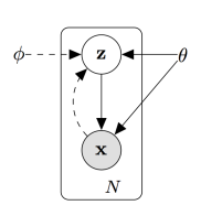
The dataset is consisting of i.i.d. samples of some continuous or discrete variable . is an unobserved continuous random variable generating the data (solid lines: ), where is the parameter set involved in the generative model. The ultimate task is to learn both and . A general method to solve such a problem is to marginalize out  to get the marginal likelihood , and maximize this likelihood  to learn . However, in many application cases, e.g. a neural network with a nonlinear hidden layer, the integral is intractable. In order to overcome this intractability, sampling-based methods, e.g. Monte Carlo EM, are introduced. But when the dataset is large, batch optimization is too costly and sampling loop per datapoint is very expensive. Therefore, the paper introduced a stochastic variational inference and learning algorithm that scales to large datasets and, under some mild differentiability conditions, even works in the intractable case.

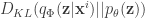
First, they defined a recognition model : an approximation to the intractable true posterior , which is interpreted as a probabilistic encoder (dash line in the directed graph), and correspondingly,  is the probabilistic decoder. Given the recognition model, the variational lower bound is defined as

In the paper’s setting,

, 

Therefore, has an analytical form. The major tricky term is the expectation which usually doesn’t have any closed solution. The usual Monte Carlo estimator for this type of problem exhibits very high variance and is not capable to take derivatives w.r.t. . Given such a problem, the paper proposed a reparameterization trick of the expectation term yields a lower bound estimator that can be straightforwardly optimized using standard stochastic gradient methods.

The key reparameterization trick constructs samples in two steps:

1. (random seed independent of )
2.   (differentiable perturbation)

such that (the correct distribution). This yields an estimator which typically has less variance than the generic estimator:

where and

A connection with auto-encoders becomes clear when looking at the objective function. The first term is the KL divergence of the approximate posterior from the prior acts as a regularizer, while the second term is a an expected negative reconstruction error.

In the experiment, they set to be a Bernoulli or Gaussian MLP, depending on the type of data they are modeling. They presented the comparisons of their method to the wake-sleep algorithm and Monte Carlo EM on MNIST and Frey Face datasets.

Overall, I think their contributions are two-fold. First, the reparameterization of the variational lower bound yields a lower bound estimator that can be straightforwardly optimized using standard stochastic gradient methods. Second, they showed that for i.i.d. datasets with continuous latent variables per datapoint, posterior inference can be made especially efficient by fitting an approximate inference model (also called a recognition model) to the intractable posterior using the proposed lower bound estimator. The stochastic gradient method helps to parallelize the algorithm so as to improve the efficiency in largescale dataset.

 

 

Deep Exponential Families

In this week’s lab meeting, I presented:

Deep Exponential Families
Rajesh Ranganath, Linpeng Tang, Laurent Charlin and David Blei.
http://arxiv.org/abs/1411.2581

This paper describes a class of latent variable models inspired by deep neural net and hierarchical generative model, called Deep Exponential Families (DEFs). DEFs stack multiple layers of exponential families and connects them with certain link functions to capture the hierarchy of dependencies.

Fast Kronecker trick for Gaussian Process regression with “expressive” kernels

On May 11th, I presented the following paper in lab meeting:

Fast Kernel Learning for Multidimensional Pattern Extrapolation
Andrew Gordon Wilson, Elad Gilboa, Arye Nehorai and John P. Cunningham

This paper presents a method for scaling up structured spectral mixture (SM) kernels (from Wilson et al 2013) for Gaussian Process regression to multi-dimensional settings in which many (but not all) of the input points live on a grid (e.g., a 2D image in which some pixels are missing).  The spectral mixture is a very expressive kernel that enhances representation learning, but the problem comes in applying it to large scale data.

Dynamic mode decomposition for large-scale neuron activity

On March 23th, I presented the following paper in lab meeting:

• Extracting spatial-temporal coherent patterns in large-scale neural recordings using dynamic mode decomposition
  Bingni W. Brunton, Lise A. Johnson, Jeffrey G. Ojemann, J. Nathan Kutz  arXiv.org

The purpose of the paper is to describe dynamic mode decomposition (DMD), a method from applied mathematics for dimensionality reduction of dynamical systems, and adapt it to the analysis of large-scale neural recordings.

Fast Marginal Likelihood Maximisation for Sparse Bayesian Models

In this week’s lab meeting, we read “Fast Marginal Likelihood Maximisation for Sparse Bayesian Models, by Tipping & Faul (2003). This paper proposes a highly accelerated algorithm for performing maximum marginal likelihood (or “evidence optimization”) in a sparse linear model (also known as the Relevance vector machine).