Deep kernel with recurrent structure

This week in lab meeting, we discussed the following work:

Learning Scalable Deep Kernels with Recurrent Structure
Al-Shedivat, Wilson, Saatchi, Hu, & Xing, JMLR 2017

This paper addressed the problem of learning a regression function that maps sequences to real-valued target vectors. Formally, the sequences of inputs are vectors of measurements , , …, , where , are indexed by time and would be of growing lengths. Let , , be a collection of the corresponding real-valued target vectors. Assuming that only the most recent steps of a sequence are predictive of the targets, the sequences can be written as , . The goal is to learn a function, , based on the available data. The approach to learning the mapping function is to use Gaussian process.

The Gaussian process (GP) is a Bayesian nonparametric model that generalizes the Gaussian distributions to functions. They assumed the mapping function is sampled from a GP. Then a standard GP regression would be performed to learn as well as the posterior predictive distribution over . The inputs to the GP are and the output function values are  . However, standard kernels, e.g. RBF, Matern, or periodic kernel, are not able to take input variables with varying length. Moreover, standard kernels won’t fully utilize the structure in an input sequence.  Therefore, this paper proposed to use recurrent models to convert an input sequence to a latent representation , then map  to . Formally, a recurrent model expresses the mapping as:

Combining the recurrent model with GP, the idea of deep kernel with recurrent model is that let be a deterministic transformation, which is a recurrent model, mapping to . Sequential structure in is integrated into the corresponding latent representations. Then a standard GP regression can be performed with input  and output .

If we denote to be the kernel over the sequence space, and  to be the kernel defined on the latent space , then

  where denotes the covariance between and  in GP.

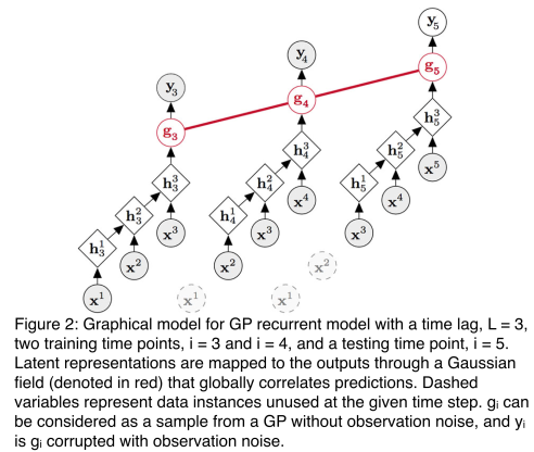
By now deep kernel with general recurrent structure has been constructed. With respect to recurrent model, there are multiple choices. Recurrent neural networks (RNNs) model recurrent processes by using linear parametric maps followed by nonlinear activations. A major disadvantage of the vanilla RNNs is that their training is nontrivial due to the so-called vanishing gradient problem: the error back-propagated through t time steps diminishes exponentially which makes learning long-term relationships nearly impossible. Thus in their paper, they chose the long short-term memory (LSTM) mechanism as the recurrent model. LSTM places a memory cell into each hidden unit and uses differentiable gating variables. The gating mechanism not only improves the flow of errors through time, but also, allows the the network to decide whether to keep, erase, or overwrite certain memorized information based on the forward flow of inputs and the backward flow of errors. This mechanism adds stability to the network’s memory. Therefore, their final model is a combination of GP and LSTM, named as GP-LSTM.

To solve the model, they needed to infer two sets of parameters: the base kernel hyperparameters, , and the parameters of the recurrent neural transformation, denoted . In order to update , the algorithm needs to invert the entire kernel matrix which requires the full dataset. However, once the kernel matrix is fixed, update of turns into a weighted sum of independent functions of each data point. One could compute a stochastic update for on a mini-batch of training points by only using the corresponding sub-matrix of . Hence, they proposed to optimize GPs with recurrent kernels in a semi-stochastic fashion, alternating between updating the kernel hyperparameters, , on the full data first, and then updating the weights of the recurrent network, , using stochastic steps. Moreover, they observed that when the stochastic updates of are small enough, does not change much between mini-batches, and hence they can perform multiple stochastic steps for before re-computing the kernel matrix, , and still converge. The final version of the optimization algorithm is given as follows:

To evaluate their model, they applied it to a number of tasks, including system identification, energy forecasting, and self-driving car applications. Quantitatively, the model was assessed on the data ranging in size from hundreds of points to almost a million with various signal-to-noise ratios demonstrating state-of-the-art performance and linear scaling of their approach. Qualitatively, the model was tested on consequential self-driving applications: lane estimation and lead vehicle position prediction. Overall, I think this paper achieved state-of-the-art performance on consequential applications involving sequential data, following straightforward and scalable approaches to building highly flexible Gaussian process.